The climate system is too complex for the human brain to grasp with simple insight. No scientist managed to devise a page of equations that explained the global atmosphere's operations. With the coming of digital computers in the 1950s, a small American team set out to model the atmosphere as an array of thousands of numbers. The work spread during the 1960s as computer modelers began to make decent short-range predictions of regional weather. Modeling long-term climate change for the entire planet, however, was held back by lack of computer power, ignorance of key processes such as cloud formation, inability to calculate the crucial ocean circulation, and insufficient data on the world's actual climate. By the mid 1970s, enough had been done to overcome these deficiencies so that Syukuro Manabe could make a quite convincing calculation. He reported that the Earth's average temperature should rise a few degrees if the level of carbon dioxide gas in the atmosphere doubled. This was confirmed in the following decade by increasingly realistic models. Skeptics dismissed them all, pointing to dubious technical features and the failure of models to match some kinds of data. By the late 1990s these problems were largely resolved, and most experts found the predictions of overall global warming convincing. Yet modelers could not be sure that the real climate would not deviate significantly from their projections as the world warmed beyond anything in the historical record. The greatest uncertainty was future changes in clouds, influenced by both warming and human emissions of aerosol particles. Incorporating ever more factors that influenced climate into elaborate "Earth System Models” brought only modest gains; modelers remained unable to say confidently whether continued greenhouse gas emissions would bring global catastrophe before the end of the 21st century, or only serious harm. (The history of rudimentary physical models without extensive calculations is told in a separate essay on Simple Models of Climate, and there is a supplementary essay for the Basic Radiation Calculations that became part of the technical foundation of comprehensive calculations.)(1)
"Dr. Richardson said that the atmosphere resembled London for in both there were always far more things going on than anyone could properly attend to."(2)
| Climate is governed by the general circulation of the atmosphere — the global pattern of air movements, with its semi-tropical trade winds, its air masses rising in the tropics to descend farther north, its cyclonic storms that carry energy and moisture through middle latitudes, and so forth. It is a vast thermodynamic engine operating to transfer heat energy from the tropics toward the poles. Many meteorologists suspected that shifts in this pattern were a main cause of climate change. They could only guess about such shifts, for the general circulation was poorly mapped before the 1940s (even the jet streams remained to be discovered). The Second World War and its aftermath brought a phenomenal increase in observations from ground level up to the stratosphere, which finally revealed all the main features. Yet up to the 1960s, the general circulation was still only crudely known, and this knowledge was strictly observational. | - LINKS -
|
| From the 19th century forward, many scientists had attempted to explain the general pattern by applying the laws of the physics of gases to a heated, rotating planet. All their ingenious efforts failed to derive a realistic mathematical solution. The best mathematical physicists could only offer simple arguments for the character of the circulation, arguments which might seem plausible but in fact were mere hand-waving.(3) And with the general global circulation not explained, attempts to explain climate change in terms of shifts of the pattern were less science than story-telling. | Full discussion in
|
| The solution would come by taking the problem from the other end. Instead of starting with grand equations for the planet as a whole, one might seek to find how the circulation pattern was built up from the local weather at thousands of points. But the physics of local weather was also a formidable problem. | |
| Early in the 20th century a Norwegian meteorologist, Vilhelm Bjerknes, argued that weather forecasts could be calculated from the basic physics of the atmosphere. He developed a set of seven "primitive equations" describing the behavior of heat, air motion, and moisture. The solution of the set of equations would, in principle, describe and predict large-scale atmospheric motions. Bjerknes proposed a "graphical calculus," based on weather maps, for solving the equations. His methods were used and developed until the 1950s, but the slow speed of the graphical calculation methods sharply limited their success in forecasting. Besides, there were not enough accurate observational data to begin with.(4) | |
| In 1922, the British mathematician and physicist Lewis Fry Richardson published a more complete numerical system for weather prediction. His idea was to divide up a territory into a grid of cells, each with its own set of numbers describing its air pressure, temperature, wind velocity, and so forth as measured at a given hour. He would then solve the equations that told how air behaved (using a method that mathematicians called finite difference solutions of differential equations). He could calculate wind speed and direction, for example, from the difference in pressure between two adjacent cells. These techniques were basically what computer modelers would eventually employ. Richardson used simplified versions of Bjerknes's "primitive equations," reducing the necessary arithmetic computations to a level where working out solutions by hand seemed feasible. Even so, "the scheme is complicated," he admitted, "because the atmosphere itself is complicated." | |
| The number of required computations was so great that Richardson scarcely hoped his idea could lead to practical weather forecasting. Even if someone assembled a "forecast-factory" employing tens of thousands of clerks with mechanical calculators, he doubted they would be able to compute weather faster than it actually happens. But if he could make a model of a typical weather pattern, it could show meteorologists how the weather worked. | |
| So Richardson attempted to compute how the weather over Western Europe had developed during a single eight-hour period, starting with the data for a day when scientists had coordinated balloon-launchings to measure the atmosphere simultaneously at various levels. The effort cost him six weeks of pencil-work (done in 1917 as a relief from his duties as an ambulance-driver amid the horrors of the Western Front). The effort ended in complete failure. At the center of Richardson's simulacrum of Europe, the computed barometric pressure climbed far above anything ever observed in the real world. | |
| Richardson suspected (rightly, as a modern review found) that the weather observations he had started with were simply not comprehensive and accurate enough for his purpose. It was the first case of what computer people would later call "garbage in, garbage out," a warning that progress in computation would always be a step behind progress in observational data. "Perhaps some day in the dim future it will be possible to advance the calculations faster than the weather advances," Richardson wrote wistfully. "But that is a dream." Taking the warning to heart, meteorologists gave up any hope of numerical modeling.(5) |
|
| Numerical Weather Prediction (1945-1955)
TOP OF PAGE |
|
| The alternative to the failed numerical approach was to keep trying to find a solution in terms of mathematical functions — a few pages of equations that an expert might comprehend as easily as a musician reads music. Through the 1950s, some leading meteorologists tried a variety of such approaches, working with simplified forms of the primitive equations that described the entire global atmosphere. They managed to get mathematical models that reproduced some features of atmospheric layers, but they were never able to convincingly show the features of the general circulation — not even something as simple and important as the trade winds. The proposed solutions had instabilities. They left out eddies and other features that evidently played crucial roles. In short, the real atmosphere was too complex to pin down in a few hundred lines of mathematics. "There is very little hope," climatologist Bert Bolin declared in 1952, "for the possibility of deducing a theory for the general circulation of the atmosphere from the complete hydrodynamic and thermodynamic equations."(6) |
|
| That threw people back on Richardson's program of numerical computation. What had been hopeless with pencil and paper might possibly be made to work with the new digital computers. A handful of extraordinary machines, feverishly developed during the Second World War to break enemy codes and to calculate atomic bomb explosions, were leaping ahead in power as the Cold War demanded ever more calculations. In the lead, energetically devising ways to simulate nuclear weapons explosions, was the Princeton mathematician John von Neumann. Von Neumann saw parallels between his explosion simulations and weather prediction (both are problems of non-linear fluid dynamics). In 1946, soon after his pioneering computer ENIAC became operational, he began to advocate using computers for numerical weather prediction.(7) |
|
| This was a subject of keen interest to everyone, but particularly to the military services, who well knew how battles could turn on the weather. Von Neumann, as a committed foe of Communism and a key member of the American national security establishment, was also concerned about the prospect of "climatological warfare." It seemed likely that the U.S. or the Soviet Union could learn to manipulate weather so as to harm their enemies. |
<=Climate mod |
| Under grants from the Weather Bureau, the Navy, and the Air Force, von Neumann assembled a small group of theoretical meteorologists at Princeton's Institute for Advanced Study. (Initially the group was at the Army's Aberdeen Proving Grounds, and later it also got support from the U.S. Atomic Energy Commission.) If regional weather prediction proved feasible, the group planned to move on to the extremely ambitious problem of modeling the entire global atmosphere. Von Neumann invited Jule Charney, an energetic and visionary meteorologist, to head the new Meteorology Group. Charney came from Carl-Gustaf Rossby's pioneering meteorology department at the University of Chicago, where the study of weather maps and fluids had developed a toolkit of sophisticated mathematical techniques and an intuitive grasp of basic weather processes. |
|
| Richardson's equations were the necessary starting-point, but Charney had to simplify them if he hoped to run large-scale calculations in weeks rather than centuries. Solutions for the atmosphere equations were only too complete. They even included sound waves (random pressure oscillations, amplified through the computations, were a main reason Richardson's heroic attempt had failed). Charney explained that it would be necessary to "filter out" these unwanted solutions, as one might use an electronic filter to remove noise from a signal, but mathematically. |
|
| Charney began with a set of simplified equations that described the flow of air along a narrow band of latitude. By 1949, his group had results that looked fairly realistic — sets of numbers that you could almost mistake for real weather diagrams, if you didn't look too closely. In one characteristic experiment, they modeled the effects of a large mountain range on the air flow across a continent. Modeling was taking the first steps toward the computer games that would come a generation later, in which the player acts as a god: raise up a mountain range and see what happens! Soon the group proceeded to fully three-dimensional models for a region.(8) | <=Radiation math |
| All this was based on a few equations that could be written on one sheet of paper. It would be decades before people began to argue that modelers were creating an entirely new kind of science; to Charney, it was just an extension of normal theoretical analysis. "By reducing the mathematical difficulties involved in carrying a train of physical thought to its logical conclusion," he wrote, "the machine will give a greater scope to the making and testing of physical hypotheses." Yet in fact he was not using the computer just as a sort of giant calculator representing equations. With hindsight we can see that computer models conveyed insights in a way that could not come from physics theory, nor a laboratory setup, nor the data on a weather map, but in an altogether new way.(9) | |
| The big challenge was still what it had been in the traditional style of physics theory: to combine and simplify equations until you got formulas that gave sensible results with a feasible amount of computation. To be sure, the new equipment could handle an unprecedented volume of computations. However, the most famous computers of the 1940s and 1950s were dead slow by comparison with a simple laptop computer of later years. Moreover, a team had to spend a good part of its time just fixing the frequent breakdowns. A clever system of computation could be as helpful as a computer that ran five times faster. Developing usable combinations and approximations of meteorological variables took countless hours of work, and a rare combination of mathematical ingenuity and physical insight. And that was only the beginning. | |
| To know when you were getting close to a realistic model, you had to compare your results with the actual atmosphere. To do that you would need an unprecedented number of measurements of temperature, moisture, wind speed, and so forth for a large region — indeed for the whole planet, if you wanted to check a global model. During the war and after, networks had been established to send up thousands of balloons that radioed back measurements of the upper air. This was largely to meet military needs, and later to help civilian aviation. For the first time the atmosphere was seen not as a single layer, as represented by a surface map, but in its full three dimensions. By the 1950s, the weather over continental areas, up to the lower stratosphere, was being mapped well enough for comparison with results from rudimentary models.(10) | |
| The first serious weather simulation that Charney's team completed was two-dimensional. They ran it on the ENIAC in 1950. Their model, like Richardson's, divided the atmosphere into a grid of cells; it covered North America with 270 points about 700 km apart. Starting with real weather data for a particular day, the computer solved all the equations for how the air should respond to the differences in conditions between each pair of adjacent cells. Taking the outcome as a new set of weather data, it stepped forward in time (using a step of three hours) and computed all the cells again. The authors remarked that between each run it took them so long to print and sort punched cards that "the calculation time for a 24-hour forecast was about 24 hours, that is, we were just able to keep pace with the weather." (A 21st-century mobile phone could do the computation in less than one second.) The resulting forecasts were far from perfect, but they turned up enough features of what the weather had actually done on the chosen day to justify pushing forward.(11) | |
| The Weather Bureau and units of the armed forces established a Joint Numerical Weather Prediction Unit, which in May 1955 began issuing real-time forecasts in advance of the weather.(12) They were not the first: since December 1954 a meteorology group at the University of Stockholm had been delivering forecasts to the Royal Swedish Air Force Weather Service, sometimes boasting better accuracy than traditional methods.(13) At their best, these models could give fairly good forecasts up to three days ahead. Yet with the limited computing power available, they had to use simplifying assumptions, not the full "primitive equations" of Bjerknes and Richardson. Even with far faster computers, the teams would have been limited by their ignorance about many features of weather, such as how clouds are formed. It would be well over a decade before the accuracy of computer forecasts began to reliably outstrip the subjective guesswork of experienced human forecasters.(14) | |
| These early forecasting models were regional, not global in scale. Calculations for numerical weather prediction were limited to what could be managed in a few hours by the rudimentary digital computers — banks of thousands of glowing vacuum tubes that frequently burned out, connected by spaghetti-tangles of wiring. Real-time weather forecasting was also limited by the fact that a computation had to start off with data that described the actual weather at a given hour at every point in a broad region. That was always far from perfect, for the instruments that measured weather were often far apart and none too reliable. Besides, the weather had already changed by the time you could bring the data together and convert it to a digital form that the computers could chew on. It was not for practical weather prediction that meteorologists wanted to push on to model the entire general circulation of the global atmosphere. | |
| The scientists could justify the expense by claiming that their work might eventually show how to alter a region’s climate for better or worse, as in von Neumann's project of climatological warfare. Perhaps some of them also hoped to learn what had caused the climate changes known from the past, back to the great Ice Ages. Some historians believed that past civilizations had collapsed because of climate changes, and it might be worth knowing about that for future centuries. But for the foreseeable future the scientists' interest was primarily theoretical: a hope of understanding at last how the climate system worked. | |
| That was a fundamentally different type of problem from forecasting. Weather prediction is what physicists call an "initial conditions" problem, where you start with the particular set of conditions found at one moment and compute how the system evolves, getting less and less accurate results as you push forward in time. Calculating the climate is a "boundary value" problem, where you define a set of unchanging conditions, the physics of air and sunlight and the geography of mountains and oceans, and compute the unchanging average of the weather that these conditions determine. | |
| The computer teams that were now arising to predict daily weather needed software code focused on hourly changes in regions the size of a county; the climate teams took a different path, developing programs for seasonal averages across the entire globe. Yet both started with the same fundamental physics equations for air and moisture. Over the following decades, weather prediction and climate teams often exchanged ideas and code for individual computation techniques and weather features. The two paths would converge in the 21st century when computers became powerful enough to handle prodigiously large calculations. At the outset, however, theoretical meteorologists could not even compute something resembling the present average global climate. That computation became their holy grail. | |
| The First General Circulation Models (1955-1965) TOP OF PAGE |
|
| Norman Phillips in Princeton took up the challenge. He was encouraged by "dishpan" experiments carried out in Chicago, where patterns resembling weather had been modeled in a rotating pan of water that was heated at the edge. For Phillips this proved that "at least the gross features of the general circulation of the atmosphere can be predicted without having to specify the heating and cooling in great detail." If such an elementary laboratory system could model a hemisphere of the atmosphere, shouldn't a computer be able to do as well? To be sure, the computer at Phillips's disposal was as primitive as the dishpan (its RAM held all of five kilobytes of memory and its magnetic drum storage unit held ten). So his model had to be extremely simple. By mid-1955 Phillips had developed improved equations for a two-layer atmosphere. To avoid mathematical complexities, his grid covered not a hemisphere but a cylinder, 17 cells high and 16 in circumference. He drove circulation by putting heat into the lower half, somewhat like the dishpan experimenters only with numbers rather than an electrical coil. The calculations turned out a plausible jet stream and the evolution of a realistic-looking weather disturbance over as long as a month. |
|
| This settled an old controversy over what processes built the pattern of circulation. For the first time scientists could see, among other things, how giant eddies spinning through the atmosphere played a key role in moving energy and momentum from place to place. Phillips's model was quickly hailed as a "classic experiment" — the first true General Circulation Model (GCM).(15) | |
| Von Neumann immediately called a conference to publicize Phillips's triumph, drumming up government funding for a long-term project. The effort got underway that same year, 1955, under the direction of Joseph Smagorinsky at the U.S. Weather Bureau near Washington, DC. Smagorinsky's goal was the one first envisaged by von Neumann and Charney: a general circulation model of the entire three-dimensional global atmosphere built directly from the primitive equations. In 1958, Smagorinsky invited Syukuro ("Suki") Manabe to join the lab. (Smagorinsky recalled that Manabe's name caught his eye when he noticed that "it didn't so much appear on papers that he had written, but on papers that his colleagues had written where they were crediting him with some of the basic ideas.") Manabe was one of a group of young men who had studied physics at Tokyo University in the difficult years following the end of the Second World War. These ambitious and independent-minded students had few opportunities for advancement in impoverished Japan, and several wound up as meteorologists in the United States. With Smagorinsky and others, Manabe would build one of the world's most vigorous and long-lasting GCM development programs.(16) |
|
| Smagorinsky and Manabe put into their model how radiation passing through the atmosphere was impeded not only by water vapor but also by ozone and carbon dioxide gas (CO2), they put in how the air exchanged water and heat with simplified ocean, land, and ice surfaces, they put in the way rain fell on the surface and evaporated or ran off in rivers, and much more. Manabe spent many hours in the library studying such esoteric topics as how various types of soil absorbed water. The huge complexities of the modeling required contributions from several others. "This venture has demonstrated to me," Smagorinsky wrote, "the value if not the necessity of a diverse, imaginative, and dedicated working group in large research undertakings." As decades passed this necessity would drive the community of researchers to grow by orders of magnitude without ceasing to collaborate closely. | |
| By 1965 Manabe's group had a reasonably complete three-dimensional model that solved the basic equations for a global atmosphere divided into nine levels (or quasi-global: they saved precious computing time by modeling only one hemisphere). This was still highly simplified, with no geography — land and ocean were blended into a single damp surface, which exchanged moisture with the air but could not take up heat. Nevertheless, the way the model moved water vapor around the planet looked gratifyingly realistic. The printouts showed a stratosphere, a zone of rising air near the equator (creating the doldrums, a windless zone that becalmed sailors), a subtropical band of deserts, and so forth. Many details came out wrong, however.(17) | |
| From the early 1960s on, modeling work interacted crucially with fields of geophysics such as hydrology (soil moisture and runoff), glaciology (ice sheet formation and flow), meteorological physics (cloud formation and precipitation, exchanges between winds and waves, and so forth). Studies of local small-scale phenomena — often stimulated by the needs of modelers — provided basic parameters for GCM's. Those developments are not covered in these essays. | <=External input |
| In the late 1950s, as computer power grew and the need for simplifying assumptions diminished, other scientists around the world began to experiment with many-leveled models based on the primitive equations of Bjerknes and Richardson. An outstanding case was the work of Yale Mintz in the Department of Meteorology of the University of California, Los Angeles (UCLA). Already in the early 1950s Mintz had been trying to use the temperamental new computers to understand the circulation of air — "heroic efforts" (as a student recalled) "during which he orchestrated an army of student helpers and amateur programmers to feed a prodigious amount of data through paper tape to SWAC, the earliest computer on campus."(18) Phillips’s pioneering 1956 paper convinced Mintz that numerical models would be central to progress in meteorology. He embarked on an ambitious program (far too ambitious for one junior professor, grumbled some of his colleagues). Unlike Smagorinsky's team, Mintz sometimes had to scramble to get access to enough computer time.(19) But like Smagorinsky, Mintz had the rare vision and drive necessary to commit himself to a research program that must take decades to reach its goals. And like Smagorinsky, Mintz recruited a young Tokyo University graduate, Akio Arakawa, to help design the mathematical schemes for a general circulation model. In the first of a number of significant contributions, Arakawa devised a novel and powerful way to represent the flow of air on a broad scale without requiring an impossibly large number of computations. |
|
| A supplementary essay on Arakawa's Computation Device describes his scheme for computing fluid flow, a good example of how modelers developed important (but sometimes controversial) techniques. | |
| From 1961 on, Mintz and Arakawa worked away at their problem, constructing a series of increasingly sophisticated GCMs. By 1964 they had simulated a climate for an entire globe, a toy planet with realistic geography — the topography of mountain ranges was there, and a rudimentary treatment of oceans and ice cover. However, that meant that with the available computer time they could compute only two layers of atmosphere against Manabe and Smagorinsky's nine. The results missed some features of the real world's climate, but the basic wind patterns and other features came out more or less right. The model, packed with useful techniques, had a powerful influence on other groups.(20*) |
|
| Arakawa was becoming especially interested in a problem that was emerging as a main barrier to progress — accounting for the effects of clouds. You don't need to spend much time looking at clouds to understand how complicated and capricious they are. The smallest single cell in a global model that a computer can handle, even today, is far larger than an individual cumulus cloud. Thus the computer calculates none of the cloud's details. Models had to get by with a "parameterization," a scheme using a set of numbers (parameters) representing the net behavior of all the clouds in a cell under given conditions. That was tricky. For example, in some of the early models the entire cloud cover "blinked" on and off in a given grid cell as the average value for humidity or the like went slightly above or below a critical threshold. Through the decades, Arakawa and others would spend countless hours developing and exchanging ways to attack the problem of representing clouds correctly.(21) |
|
| Modeling techniques and entire GCMs spread by a variety of means. In the early days, as Phillips recalled, modelers had been like "a secret code society." The machine-language computer programs were "an esoteric art which would be passed on in an apprentice system."(22) Over the years, programming languages became more transparent and codes were increasingly well documented. Yet there were so many subtleties that a real grasp still required an apprenticeship on a working model. Commonly, a new modeling group began with some version of another group's model. A post-doctoral student (especially from the influential UCLA group) might take a job at another institution, bringing along his old team's computer code. The new team he assembled would start off working with the old code and then set to modifying it. Others built new models from scratch. Through the 1960s and 1970s, important GCM groups emerged at institutions from New York to Australia. |
|
| Americans dominated the field during the first postwar decades. That was assured by the government funding that flowed into almost anything related to geophysics, computers, and other subjects likely to help in the Cold War. The premier group was Smagorinsky's Weather Bureau unit (renamed the Geophysical Fluid Dynamics Laboratory in 1963), with Manabe's groundbreaking models. In 1968, the group moved from the Washington, DC area to Princeton, and it eventually came under the wing of the U.S. National Oceanic and Atmospheric Administration. Almost equally influential were the Mintz-Arakawa group at UCLA. Another major effort got underway in 1964 at the National Center for Atmospheric Research (NCAR) in Boulder, Colorado under Warren Washington and yet another Tokyo University graduate, Akira Kasahara. The framework of their first model was quite similar to Richardson’s pioneering attempt, but without the instability that had struck him down, and incorporating additional features such as the transfer of radiation up and down through the atmosphere — or rather between the two vertical layers that was all their computer could handle. |
|
| Less visible was a group at RAND Corporation, a defense think-tank in California. Their studies, based on the Mintz-Arakawa model, were driven by the Department of Defense's concern about possibilities for deliberately changing a region's climate. Although the RAND results were published only in secret "gray" reports, the work produced useful techniques that became known to other modelers. Meanwhile Charles Leith at another defense-oriented facility, the Lawrence Livermore National Laboratory in California, devised a model to play with on what was then the world's fastest computer. Leith soon moved on to other work without writing a publication, but his colored movies of the model's output of weather patterns impressed his peers.(23) |
|
| Many Kinds of Models TOP OF PAGE | |
| Although the modelers of the 1950s and early 1960s got results good enough to encourage them to persevere, they were still a long way from reproducing the details of the Earth's actual circulation patterns and its regions of drought or rainfall. Thoughts of investigating climate change scarcely entered their minds; their goal was basic atmospheric science, to understand fundamental processes like the trade winds and jet streams. In 1965, a blue-ribbon panel of the U.S. National Academy of Sciences reported on where GCMs stood that year. The panel reported that the best models (like Mintz-Arakawa and Smagorinsky-Manabe) calculated simulated atmospheres with gross features "that have some resemblance to observation." There was still much room for improvement in converting equations into systems that a computer could work through within a few weeks. To do much better, the panel concluded, modelers would need computers that were ten or even a hundred times more powerful.(24) | |
| Yet even if the computers had been vastly faster, the simulations would still have been unreliable. For they were running up against that famous limitation of computers, "garbage in, garbage out." Some sources of error were known but hard to drive out, such as getting the right parameters for factors like convection in clouds. To diagnose the failings that kept GCMs from being more realistic, scientists needed an intensified effort to collect and analyze aerological data — the actual profiles of wind, heat, moisture, and so forth, at every level of the atmosphere and all around the globe. The data in hand were still deeply insufficient. Continent-scale weather patterns had been systematically recorded only for the Northern Hemisphere's temperate and arctic regions and only since the 1940s; the vast South Pacific and Southern Ocean in particular were like the blank spaces on ancient maps that cartographers could only decorate with imaginary beasts. Through the 1960s, the actual state of the entire general circulation remained unclear. For example, the leisurely vertical movements of air had not been measured at all, so the large-scale circulation could only be inferred from the horizontal winds. As for the atmosphere's crucial water balance and energy balance, one expert estimated that the commonly used numbers might be off by as much as 50%.(25) Smagorinsky put the problem succinctly in 1969: "We are now getting to the point where the dispersion of simulation results is comparable to the uncertainty of establishing the actual atmospheric structure."(26) |
|
| In the absence of a good match between atmospheric data and GCM calculations, many researchers continued through the 1960s to experiment with simple models for climate change. A few equations and some hand-waving gave a variety of fairly plausible descriptions for how one or another factor might cause an ice age or global warming. There was no way to tell which of these models was correct, if any. As for the present circulation of the atmosphere, some continued to work on pencil-and-paper mathematical models that would represent the planet's shell of air with a few fundamental physics equations, seeking an analytic solution that would bypass the innumerable mindless computer operations. They made little headway. In 1967, Edward Lorenz, an MIT professor of meteorology, cautioned that "even the trade winds and the prevailing westerlies at sea level are not completely explained." Another expert more bluntly described where things stood for an explanation of the general circulation: "none exists." Lorenz and a few others began to suspect that the problem was not merely difficult, but impossible in principle. Climate was apparently not a well-defined system, but only an average of the ever-changing jumble of daily thunderstorms and storm fronts.(27) |
|
| Would computer modelers ever be able to say they had "explained" the general circulation? Many scientists looked askance at the new method of numerical simulation as it crept into more and more fields of research. This was not theory, and it was not observation either; it was off in some odd new country of its own. People were attacking many kinds of scientific problems by taking a set of basic equations, running them through hundreds of thousands of computations, and publishing a result that claimed to reflect reality. Their results, however, were simply stacks of printout with rows of numbers. That was no "explanation" in the traditional sense of a model in words or diagrams or equations, something you could write down on a few pages, something your brain could grasp intuitively as a whole. The numerical approach "yields little insight," Lorenz complained. "The computed numbers are not only processed like data but they look like data, and a study of them may be no more enlightening than a study of real meteorological observations."(28) | |
| Yet the computer scientist could "experiment" in a sense, by varying the parameters and features of a numerical model. You couldn't put a planet on a laboratory bench and vary the sunlight or the way clouds were formed, but wasn't playing with computer models functionally equivalent? In this fashion you could make a sort of "observation" of almost anything, for example, the effect of changing the amount of moisture or CO2 in the atmosphere. Through many such trials you might eventually come to understand how the real world operated. Indeed you might be able to observe the planet more clearly in graphs printed out from a model than in the clutter of real-world observations, so woefully inaccurate and incomplete. As one scientist put it, "in many instances large-scale features predicted by these models are beyond our intuition or our capability to measure in the real atmosphere and oceans."(29) | |
| Sophisticated computer models were gradually displacing the traditional hand-waving models where each scientist championed some particular single "cause" of climate change. Such models had failed to come anywhere near to explaining even the simplest features of the Earth's climate, let alone predicting how it might change. A new viewpoint was spreading along with digital computing. Climate was not regulated by any single cause, the modelers said, but was the outcome of a staggeringly intricate complex of interactions, which could only be comprehended in the working-through of the numbers themselves. |
|
| GCMs were not the only way to approach this problem. Scientists were developing a rich variety of computer models, for there were many ways to slice up the total number of arithmetic operations that a computer could run through in whatever time you could afford to pay for. You could divide up the geography into numerous cells, each with numerous layers of atmosphere; you could divide up the time into many small steps, and work out the dynamics of air masses in a refined way; you could make complex calculations of the transfer of radiation through the air; you could construct detailed models for surface effects such as evaporation and snow cover... but you could not do all these at once. Different models intended for different purposes made different trade-offs. | |
| One example was the work of Julian Adem in Mexico City, who sought a practical way to predict climate anomalies a few months ahead. He built a model that had low geographical resolution but incorporated a large number of land and ocean processes. John Green in London pursued a wholly different line of attack, aimed at shorter-term weather prediction. His analysis concentrated on the actions of large eddies in the atmosphere and was confined to idealized mathematical equations. It proved useful to computer modelers who had to devise numerical approximations for the effects of the eddies. Other groups chose to model the atmosphere in one or two dimensions rather than all three.(30) The decisions such people made in choosing an approach involved more than computer time. They also had to allocate another commodity in short supply — the time they could spend thinking. | |
| This essay does not cover the entire range of models, but concentrates on those which contributed most directly to greenhouse effect studies. For models in one or two dimensions, see the article on Basic Radiation Calculations. | |
| None of the concepts of the 1960s inspired confidence. The modelers were missing some essential physics, and their computers were too slow to perform the millions of computations needed for a satisfactory solution. But as one scientist explained, where the physics was lacking, computers could do schematic "numerical experiments" directed toward revealing it.(31) By the time modelers got their equations and parameters right, surely not many years off, the computers would have grown faster by another order of magnitude or so and would be able to handle the necessary computations. In 1970, a report on environmental problems by a panel of top experts declared that work on computer models was "indispensable" for progress in the study of climate change.(32*) |
|
| The growing community of climate modelers was strengthened by the advance of computer systems that carried out detailed calculations on short timescales for weather prediction. This progress required much work on parameterization — schemes for representing cloud formation, interactions between waves and winds, and so forth. Such studies accelerated as the 1970s began.(33) The weather forecasting models also required data on conditions at every level of the atmosphere at thousands of points around the world. Such observations were now being provided by the balloons and sounding rockets of an international World Weather Watch, founded in the mid 1960s. The volume of data was so great that computers had to be pressed into service to compile the measurements. Computers were also needed to check the measurements for obvious errors (sometimes several percent of the thousands of observations needed to be adjusted). Finally, computers would massage the data with various smoothing and calibration operations to produce a unified set of numbers to feed into calculations. The instrumental systems were increasingly oriented toward producing numbers meaningful to the models, and vice-versa; global data and global models were no longer distinct entities, but parts of a single system for representing the world.(34) The weather predictions became accurate enough — looking as far as three days ahead — to be economically important. That built support for the meteorological measurement networks and computer studies necessary for climate work. |
|
| An example of the crossover could be found at NASA's Goddard Institute for Space Studies in New York City. A group there under James (Jim) Hansen had been developing a weather model as a practical application of its mission to study the atmospheres of planets. For one basic component of this model, Hansen developed a set of equations for the transfer of radiation through the atmosphere, based on work he had originally done for studies of the planet Venus. The same equations could be used for a climate model, by combining them with the elegant method for computing fluid dynamics that Arakawa had developed. |
|
| In the 1970s, Hansen assembled a team to work up schemes for cloud physics and the like to put into a model that would be both fast-running and realistic. An example of the kind of detail they pursued was a simple equation they devised to represent the reflection of sunlight from snow. They included the age of the snow layer (as it gradually melted away) and the "masking" by vegetation (snowy forests are darker than snowy tundra). To do the computations within a reasonable time, they had to use a grid with cells a thousand kilometers square, averaging over all the details of weather. Eventually they managed to get a quite realistic-looking climate. It ran an order of magnitude faster than some rival GCMs, permitting the group to experiment with multiple runs, varying one factor or another to see what changed.(35*) In such studies, the global climate was beginning to feel to researchers like a comprehensible physical system, akin to the systems of glassware and chemicals that experimental scientists manipulated on their laboratory benches. |
|
| Meanwhile the community of modelers continued to devise more realistic parameters for various physical processes, and to improve their mathematical techniques. A major innovation that appeared in the 1970s, spread rapidly, and was dominant by the 1990s, took a radically different approach to the basic architecture of models. Instead of dividing the planet's surface into a grid of thousands of square cells, teams took to dividing the globe into a tier of segments — hemispheres, quadrants, eighths, sixteenths, etc. ("spherical harmonics"). After doing a calculation on this abstracted system, they could combine and transform the numbers back into a geographical map. This "spectral transform" technique simplified many of the computations, but it was feasible only with the much faster new computers. For decades afterward, physicists who specialized in other fields of fluid dynamics were startled when they saw a climate model that did not divide up the atmosphere into millions of boxes, but used the refined abstraction of spherical harmonics. The method worked only because the Earth's atmosphere has an unusual property for a fluid system — it is in fact quite nearly spherical. | |
| The new technique was especially prized because it got around the trouble computers had with the Earth's poles, where all the lines of longitude converge in a point and the mathematics gets weird. (The earliest models had avoided the poles altogether and computed climate on a cylinder, but that wouldn't take you very far.) Spherical harmonics did not exhaust the ingenuity of climate modelers. For example, in the late 1990s, when people had begun to run separate computations for the atmospheric circulation and the equally important circulation of ocean currents, many groups introduced new coordinate schemes for their ocean models. They avoided problems with the North and South Poles simply by shifting the troublesome convergence points onto a land mass. Another example of the never-ending search for better computational techniques: some models developed in the 2010s divided the surface of the globe into six segments like the faces of an inflated cube, with artful interactions along the edges.(36) | |
| Groups continued to proliferate, borrowing ideas from earlier models and devising new techniques of their own. Here as in most fields of science, Europeans had recovered from the war's devastation and were catching up with the Americans. In particular, during the mid-1970s a consortium of nations set up a European Centre for Medium-Range Weather Forecasts and began to contribute to climate modeling. A "family tree" of relations between leading models is here. | |
| Predictions of Warming (1965-1979) TOP OF PAGE | |
| In their first decade or so of work the GCM modelers had treated climate as a given, a static condition. They had their hands full just trying to understand one year's average weather. Typical was a list that Mintz made in 1965 of possible uses for his and Arakawa's computer model. Mintz showed an interest mainly in answering basic scientific questions. He also listed long-range forecasting and "artificial climate control" — but not greenhouse effect warming or other possible causes of long-term climate change.(38) |
|
| Around this time, however, a few modelers began to take an interest in global climate change as a problem over the long term. The discovery that the level of CO2 in the atmosphere was rising fast prompted hard thinking about greenhouse warming, prompting conferences and government panels in which GCM experts like Smagorinsky participated.(39*) Computer modelers began to interact with the community of carbon researchers. Another stimulus was Fritz Möller's discovery in 1963 that simple models built out of a few equations — the only models available for long-term climate change — showed grotesque instabilities. Everyone understood that Möller's model was unrealistic (in fact it had fundamental flaws). Nevertheless it raised a nagging possibility that mild perturbations, such as humanity itself might bring about, could trigger an outright global catastrophe.(40) |
|
| Manabe took up the challenge. He had a long-standing interest in the effects of CO2, not because he was worried about the future climate, but simply because the gas at its current level was a significant factor in the planet's heat balance. But when Möller visited Manabe and explained his bizarre results, Manabe decided to look into how the climate system might change. He and his colleagues were already building a model that took full account of the movements of heat and water. To get a really sound answer, the entire atmosphere had to be studied as a tightly interacting system. In particular, Manabe's group calculated the way rising columns of moisture-laden air conveyed heat from the surface into the upper atmosphere, a crucial part of the system which most prior models had failed to incorporate. The required computations were so extensive, however, that Manabe stripped down the model to a single one-dimensional column, which represented the atmosphere averaged over the globe (or in some runs, averaged over a particular band of latitude). His aim was to get a system that could be used as a basic building-block for a full three-dimensional GCM.(41) |
|
| In 1966, Manabe and a collaborator, Richard Wetherald, used the one-dimensional model to test what would happen if the level of CO2 changed. Their target was something that would eventually become a central preoccupation of modelers: the climate's "sensitivity." Just how much would temperature be altered when something affected incoming and outgoing radiation (a change in the Sun's output of sunlight, say, or a change in CO2)? The method was transparent. Run a model with one value of the something (say, of CO2 concentration), run it again with a new value, and compare the answers. Researchers since Arrhenius had pursued this with highly simplified models. They used as a benchmark the difference if the CO2 level doubled.(42) That not only made comparisons between results easier, but seemed like a good number to look into. For it seemed likely that the level would in fact double before the end of the 21st century, thanks to humanity's ever-increasing use of fossil fuels. The answer Manabe's group came up with was that global temperature would rise roughly 2°C (around 3-4°F).(43) | |
| This was the first time a greenhouse warming computation included enough of the essential factors, in particular the effects of water vapor, to seem plausible to experts. Wallace Broecker, who would later play a major role in climate change studies, recalled that it was the 1967 paper "that convinced me that this was a thing to worry about." Another scientist called it "arguably the greatest climate-science paper of all time," for it "essentially settled the debate on whether carbon dioxide causes global warming." Experts in a 2015 poll agreed, naming it as the "most influential" of all climate change papers.(44) The work drew on all the experience and insights accumulated in the labor to design GCMs, yet it was no more than a first baby step toward a realistic three-dimensional model of the changing climate. | |
| The next important step was taken in the late 1960s by Manabe’s group, now at Princeton. Their GCM was still highly simplified. In place of actual land and ocean geography they pictured a geometrically neat planet, half damp surface (land) and half wet (a "swamp" ocean). Worse, they could not predict cloudiness but just held it unchanged at the present level when they calculated the warmer planet with doubled CO2. However, they did incorporate the movements of water, predicting changes in soil moisture and snow cover on land, and they calculated sea surface temperatures well enough to show the extent of sea ice. They computed nine atmospheric levels. The results, published in 1975, looked quite realistic overall (link from below). |
|
| The model with increased CO2 had more moisture in the air, with an intensified hydrological cycle of evaporation and precipitation. That was what physicists might have expected for a warmer atmosphere on elementary physical grounds (if they had thought about it, which few had). Actually, with so many complex interactions between soil moisture, cloudiness, and so forth, a simple argument could be in error. It took the model computation to show that this accelerated cycle really could happen, as hot soil dried out in one region and more rain came down elsewhere. The Manabe-Wetherald model also showed greater warming in the Arctic than in the tropics. This too could be predicted from simple reasoning. Not only did a more active circulation carry poleward more heat and more water vapor (the major greenhouse gas), but warming meant less snow and ice and thus the ground and sea would absorb more sunlight and more heat from the air. Again it took a calculation to show that what sounded reasonable on elementary principles would indeed happen in the real world (or at least in a reasonable simulation of it).(45*) | |
| Averaged over the entire planet, for doubled CO2 the computer predicted a warming of around 3.5°C. It all looked plausible. The results made a considerable impact on scientists, and through them on policy-makers and the public. | =>Government =>Public opinion = Milestone |
| Manabe and Wetherald warned that "it is not advisable to take too seriously" the specific numbers they published.(46) They singled out the way the model treated the oceans as a simple wet surface. On our actual planet, the oceans absorb large quantities of heat from the atmosphere, move it around, and release it elsewhere.(47) Another and more subtle problem was that Manabe and Wetherald had not actually computed a climate change. Instead they had run their model twice to compute two equilibrium states, one with current conditions and one with doubled CO2. In the real world, the atmosphere would pass through a series of changes as the level of the gas rose, and there were hints that the model could end up in different states depending on just what route it took. | |
| Even if those uncertainties could be cleared up, there remained the old vexing problem of clouds. As the planet got warmer the amounts of cloudiness would probably change at each level of the atmosphere in each zone of latitude, but change how? There was no reliable way to figure that out. Worse, it was not enough to have a simple number for cloud cover. Scientists were beginning to realize that clouds could either tend to cool a region (by reflecting sunlight) or warm it (by trapping heat radiation from below, especially at night). The net effect depended on the types of cloud and how high they floated in the atmosphere. A better prediction of climate change would have to wait on general improvements. |
|
| Progress was steady, thanks to the headlong advance of electronic computers. From the mid 1950s to the mid 1970s, the power available to modelers increased by a factor of thousands. That meant modelers could put in more factors in more complex ways, they could divide the planet into more segments to get higher resolution of geographical features, and they could run models to represent longer periods of time. The models no longer had gaping holes that required major innovations, and the work settled into a steady improvement of existing techniques. At the foundations, modelers devised increasingly more sophisticated and efficient schemes of computation. As input for the computations they worked endlessly to improve the parameters that assigned numbers to each process. From around 1970 on, many journal articles appeared with ideas for dealing with convection, evaporation of moisture, reflection from ice, and so forth.(48) | <=External input |
| The most essential element for progress, however, was better data on the real world. Strong efforts were rapidly extending the observing systems. For example, in 1959 the physicist Lewis Kaplan found an ingenious way to use measurements of infrared radiation from satellites to find the temperature at different levels of the atmosphere, all around the world. During the 1960s satellite data began to provide heat budgets by zones of latitude, which gave a measure of transport of heat toward the poles. "It is a warmer and darker planet than we previously believed," one report announced. "More solar energy is being absorbed, primarily in the tropics... The trend toward departure from the earlier computation studies of the radiation budget seems irreversible." In 1969 NASA's Nimbus 3 satellite began to broadcast measurements designed explicitly to provide a fundamental check on model results. The reflection of sunlight at each latitude from Manabe's 1975 model planet agreed pretty well with the actual numbers for the Earth, as measured by Nimbus 3 (see above).(48a) |
|
| Manabe's team was interacting along informal channels with several other groups. An example was a project code-named NILE BLUE, funded by the Department of Defense during 1970-1973 and interested in using climate modification as a weapon. Declassified and transferred to the National Science Foundation, the project carried out a variety of pioneering studies and helped verify the reliability of climate models. Also encouraging was a 1972 model by Mintz and Arakawa (unpublished, like much of their work), which managed to simulate in a rough way the huge changes in weather patterns as sunlight shifted from season to season. During the next few years, Manabe and collaborators published a model that produced entirely plausible seasonal variations. To modelers, the main point of such work was gaining insight into the dynamics of climate through close inspection of their printouts. (They could study, for example, just what role the ocean surface temperature played in driving the tropical rain belt from one hemisphere to the other as the seasons changed.) To everyone else, seasons were a convincing test of the models' validity. It was almost as if a single model worked for two quite different planets — the planets Summer and Winter. A 1975 review panel felt that with this success, realistic numerical climate models "may be considered to have begun."(49*) | |
| Yet basic problems such as predicting cloudiness remained unsolved, while new difficulties rose into view. For example, scientists began to realize that the way clouds formed, and therefore how much they helped to warm or cool a region, could be strongly affected by the haze of dust and chemical particles floating in the atmosphere. Little was known about how these aerosols helped or hindered the formation of different types of clouds. Another surprise came when two scientists pointed out that the reflectivity of clouds and snow depends on the angle of the sunlight — and in polar regions the Sun always struck at a low angle.(50) Figuring how sunlight might warm an ice cap was as complicated as the countless peculiar forms taken by snow and ice themselves. Little of this had been explored through physics theory. Nor had it been measured in the field, for it was only gradually that model-makers realized how much they suffered from the absence of reliable measurements of the parameters they needed to describe the action of dust particles, snow surfaces, and so forth. Overall, as Smagorinsky remarked in 1972, modelers still needed "to meet standards of simulation fidelity considerably beyond our present level."(51) |
|
| Modelers felt driven to do better, for people had begun to demand much more than a crude reproduction of the present climate. In the early 1970s the rise of environmentalism, a series of weather disasters, and the energy crisis had put greenhouse warming on the public agenda. While model research remained the key to understanding fundamental climate processes, this traditional motive was joined by a drive to produce findings that would be immediately relevant to policy-makers and the public. |
|
| It was now a matter of concern to citizens (or at least the most scientifically well-informed citizens) whether the computer models were correct in their predictions of how CO2 emissions would raise global temperatures. Newspapers reported disagreements among prominent scientists. Some experts suspected that factors overlooked in the models might keep the climate system from warming at all, or might even bring on cooling instead. "Meteorologists still hold out global modeling as the best hope for achieving climate prediction," a senior scientist observed in 1977. "However, optimism has been replaced by a sober realization that the problem is enormously complex."(52*) | |
| The problem was so vexing that the President's Science Adviser (who happened to be a geophysicist) asked the National Academy of Sciences to study the issue. The Academy appointed a panel, chaired by Jule Charney and including other respected experts who had been distant from the recent climate debates. They convened at Woods Hole in the summer of 1979. They had plenty of work to review, for by this time there were enough independent climate modeling groups to create a substantial literature. For example, a conference that convened in Washington, DC in 1978 to compare and evaluate models (the first of many "intercomparison" meetings) brought together 81 scientists from modeling groups in 10 countries.(52a) Charney's panel concentrated on comparing the two most complete GCMs, one constructed by Manabe's team and the other by Hansen's — elaborate three-dimensional models that used different physical approaches and different computational methods for many features. The panel found differences in detail but solid agreement for the main point: the world would get warmer as CO2 levels rose. |
=>Aerosols |
| But might both GCMs share some fundamental unrecognized flaw? As a basic check, the Charney Panel went back to the models of one-dimensional and two-dimensional slices of atmosphere, which various groups were using to explore a wider range of possibilities than the GCMs could handle. These models showed crudely but directly the effects of adding CO2 to the atmosphere. All the different approaches, simplified in very different ways, were in rough overall agreement. They came up with figures that were at least in the same ballpark for the temperature in an atmosphere with twice as much CO2 (the level projected for around the middle of the 21st century). Then and ever since, nobody was able to construct any kind of model that could roughly mimic the present climate and that did not get warmer when CO2 was added.(53*) |
|
| To make their conclusion more concrete, the Charney Panel decided to announce a specific range of numbers. They argued out among themselves a rough-and-ready compromise. Hansen's GCM predicted a 4°C rise for doubled CO2, and Manabe's latest figure was around 2°C. Splitting the difference, the Panel thought it "most probable" that if CO2 reached this level the planet would warm up by about three degrees, plus or minus fifty percent: in other words, 1.5–4.5°C (2.7–8°F). They concluded dryly, "We have tried but have been unable to find any overlooked or underestimated physical effects" that could reduce the warming. | =>CO2 greenhouse =>Public opinion = Milestone =>Government =>International |
| Strenuous efforts by thousands of scientists over the next half-century would bring ironclad confirmation of the Panel's audaciously specific prediction of a sensitivity of 3°C, and could not narrow the range of uncertainty. (In 2021 the "very likely" range was revised slightly up, to 2-5°C.) "What made the Charney Report so prescient?" asked a group of experts in 2011. And how could the Panel be so confident, when there was not yet a clear signal that global warming was underway? The experts concluded that an “emphasis on the importance of physical understanding gained through theory and simple models" gave the Panel "a good understanding of the main processes governing climate sensitivity." Global warming was not yet visible, but the National Academy of Sciences itself was warning that it would come.(54*) | "Three degrees of warming" means the global average. The warming is much greater at northern latitudes, and greater over land than over the oceans. |
| Ocean Circulation and Real Climates
(1969-1988) TOP OF PAGE |
|
| In the early 1980s, several groups pressed ahead toward more realistic models. They put in a reasonable facsimile of the Earth's actual geography, and replaced the wet "swamp" surface with an ocean that could exchange heat with the atmosphere. Thanks to increased computer power the models were now able to handle seasonal changes as a matter of course. It was also reassuring when Hansen's group and others got a decent match to the rise-fall-rise curve of global temperatures since the late 19th century, once they put in not only the rise of CO2 but also changes in emissions of volcanic dust and solar activity. |
<=Aerosols |
| Adding a solar influence was a stretch, for nobody had figured out any plausible way that the superficial variations seen in numbers of sunspots could affect climate. To arbitrarily adjust the strength of the presumed solar influence in order to match the historical temperature curve was guesswork, dangerously close to fudging. But many scientists suspected there truly was a solar influence, and adding it did improve the match. Sometimes a scientist must "march with both feet in the air," assuming a couple of things at once in order to see whether it all eventually works out.(55) |
|
| Other modelers had not tried to project actual global temperatures beyond the end of the century, but Hansen's team boldly pushed ahead to 2020. They calculated that by then the world would have warmed roughly another half a degree (which was what would indeed happen). From this point on climate modelers increasingly looked toward the future. When they introduced a doubled CO2 level into their improved models, they consistently found the same few degrees of warming.(56*) |
|
| The skeptics were not persuaded. The Charney Panel itself had pointed out that much more work was needed before models would be fully realistic. The treatment of clouds remained a central uncertainty. Another great unknown was the influence of the oceans. Back in 1979 the Charney Panel had surmised that the oceans' enormous capacity for soaking up heat could delay an atmospheric temperature rise for decades; global warming might not become obvious to everyone until it was too late to take timely precautions.(57) If there was such a time lag, or indeed any delayed effects due to feedbacks and lags in the system, the existing GCMs would not show it, for they computed only equilibrium states. Lacking most of the necessary data and thwarted by formidable calculational problems, the models simply could not account for the true influence of the oceans. | |
| The world-ocean is not a stagnant pool. Like the atmosphere, it is a thermodynamic engine that carries heat energy from the tropics towards the poles — much more heat than the atmosphere, but much more slowly. Ever since Benjamin Franklin discovered the Gulf Stream, people had sought to understand the ocean circulation and how it mattered for climate. By the 1960s scientists had mapped the overall pattern, but they struggled to grasp all the driving forces. |
|
| Massive international programs of data-gathering were beginning to reveal some of the problems. Oceanographers saw that simple currents like the Gulf Stream were not the only driver. Large amounts of energy were carried through the seas by a myriad of whorls of various types, from tiny convection swirls up to sluggish eddies a thousand kilometers wide. Calculating these whorls, like calculating all the world's individual clouds, was beyond the reach of the fastest computer. Again parameters had to be devised to summarize the main effects, only this time for entities that were far worse observed and worse understood than clouds. Modelers could only put in average numbers to represent the heat that they knew somehow moved vertically from layer to layer in the seas, and the energy somehow carried from warm latitudes toward the poles. They suspected that the actual behavior of the oceans might work out quite differently from their models. And even with the simplifications, to get anything halfway realistic required a vast number of computations, even more than for the atmosphere. |
<=>The oceans |
| Manabe was keenly aware that if the Earth's future climate were ever to be predicted, it was "essential to construct a realistic model of the joint ocean-atmosphere system."(58) He shouldered the task in collaboration with Kirk Bryan, an oceanographer with meteorological training, who had been brought into the group back in 1961 to build a stand-alone numerical model of the circulation of an ocean. The two got together to construct a computational system that coupled together their separate models. Manabe's winds and rain would help drive Bryan's ocean currents, while in return Bryan's sea-surface temperatures and evaporation would help drive the circulation of Manabe's atmosphere. At first they tried to divide the work: Manabe would handle matters from the ocean surface upward, while Bryan would take care of what lay below. But they found things just didn't work that way for studying a coupled system. They moved into one another's territory, aided by a friendly personal relationship. | |
| Bryan and Manabe were the first to put together in one package approximate calculations for a wide variety of important features. They not only incorporated both oceans and atmosphere, but added into the bargain feedbacks from changes in sea ice and a detailed scheme that represented, region by region, how moisture built up in the soil, evaporated, or ran off in rivers to the sea. | |
| Their big problem was that from a standing start it took several centuries of simulated time for an ocean model to settle into a realistic state. After all, that was how long it would take the surface currents of the real ocean to establish themselves from a random starting-point. The atmosphere, however, readjusts itself in a matter of weeks. After about 50,000 time steps of ten minutes each, Manabe's model atmosphere would approach equilibrium. The team could not conceivably afford the computer time to pace the oceans through decades in ten-minute steps. Their costly Univac 1108, a supercomputer by the standards of the time, needed 45 minutes to compute the atmosphere through a single day. Bryan's ocean could use longer time steps, say a hundred minutes, but the simulated currents would not even begin to settle down until millions of these steps had passed. | |
| The key to their success was a neat trick for matching the different timescales. They ran their ocean model with its long time steps through twelve days. They ran the atmosphere model with its short time-steps through three hours. Then they coupled the atmosphere and ocean to exchange heat and moisture. Back to the ocean for another twelve days, and so forth. They left out seasons, using average annual sunlight to drive the system. | |
| Manabe and Bryan were confident enough of their model to undertake a heroic computer run, some 1100 hours long (more than 12 full days of computer time devoted to the atmosphere and 33 to the ocean). In 1969, they published the results in an unusually short paper, as Manabe recalled long afterward — "and still I am very proud of it."(59) | |
| Bryan wrote modestly at the time that "in one sense the... experiment is a failure." For even after a simulated century, the deep ocean circulation had not nearly reached equilibrium. It was not clear what the final climate solution would look like.(60) Yet it was a great success just to carry through a linked ocean-atmosphere computation that was at least starting to settle into equilibrium. The result looked like a real planet — not our Earth, for in place of geography there was only a radically simplified geometrical sketch, but in its way realistic. It was obviously only a first draft with many details wrong, yet there were ocean currents, trade winds, deserts, rain belts, and snow cover, all in roughly the right places. Unlike our actual Earth, so poorly observed, in the simulation one could see every detail of how air, water, and energy moved about. |
<=>The oceans |
| Following up, in 1975 Manabe and Bryan published results from the first coupled ocean-atmosphere GCM that had a roughly Earth-like geography. Looking at their crude map, one could make out continents like North America and Australia, although not smaller features like Japan or Italy. The supercomputer ran for fifty straight days, simulating movements of air and sea over nearly three centuries. "The climate that emerges," they wrote, "includes some of the basic features of the actual climate." For example, it showed the Sahara and the American Southwest as deserts, but plenty of rain in the Pacific Northwest and Brazil. Manabe and Bryan had not shaped their equations deliberately to bring forth such features. These were "emergent features," emerging spontaneously out of the computations. The computer’s output looked roughly like the actual climate only because the modelers had succeeded in roughly representing the actual operations of the atmosphere upon the Earth’s geography. |
|
| "However," Manabe and Bryan admitted, their model had "many unrealistic features." For example, it still failed to show the full oceanic circulation. After all, the inputs had not been very realistic — for one thing, the modelers had not put in the seasonal changes of sunlight. Still, the results were getting close enough to reality to encourage them to push ahead.(61) By 1979, they had mobilized enough computer power to run their model through more than a millennium while incorporating seasons.(62) |
<=>The oceans |
| Meanwhile the team headed by Warren Washington at NCAR in Colorado developed another ocean model, based on Bryan's, and coupled it to their own quite different GCM. Since they had begun with Bryan's ocean model it was not surprising that their results resembled Manabe and Bryan's, but it was still a gratifying confirmation. Again the patterns of air temperature, ocean salinity, and so forth came out roughly correct overall, albeit with noticeable deviations from the real planet, such as tropics that were too cold. As Washington's team admitted in 1980, the work "must be described as preliminary."(63) Through the 1980s, these and other teams continued to refine coupled models, occasionally checking how they reacted to increased levels of CO2. These were not so much attempts to predict the real climate as experiments to work out methods for doing so. | |
| The results, for all their limitations, said something about the predictions of the atmosphere-only GCMs. The Charney Panel had worried that the oceans would delay the appearance of global warming for decades by soaking up heat. In 1985 Hansen's group found such a lag with a crude model, and repeated the warning that a policy of "wait and see" might be wrongheaded. A temperature rise in the atmosphere might not become obvious until much worse greenhouse warming was inevitable. (As explained below, temperature would actually stabilize promptly if the CO2 rise could be halted. But the warning was valid: by the time people were convinced that global warming was happening, delays in the world's political, economic and biological systems would make more emissions and thus further heating unavoidable.) Also as expected, complex feedbacks showed up in the ocean circulation, influencing just how the weather would change in a given region. Aside from that, including a somewhat realistic ocean did not turn up anything that would alter the basic prediction of future warming. Once again it was found that simple models had pointed in the right direction.(64) |
|
| A few of the calculations showed a disturbing new feature — a possibility that the ocean circulation was fragile. Signs of rapid past changes in circulation had been showing up in ice cores and other evidence that had set oceanographers to speculating. In 1985, Bryan and a collaborator tried out a coupled atmosphere-ocean model with a CO2 level four times higher than at present. They found signs that the world-spanning "thermohaline" circulation, where differences in heat and salinity drove a vast overturning of seawater in the North Atlantic, could come to a halt. Three years later Manabe and another collaborator produced a simulation in which, even at present CO2 levels, the ocean-atmosphere system could settle down in one of two states — the present one, or a state without the overturning.(66*) Some experts worried that global warming might indeed shut down the circulation. They feared that halting the steady flow of warm water into the North Atlantic would bring devastating climate changes in Europe and perhaps beyond. |
|
| Oceanographer Wallace Broecker remarked that the early GCMs had been designed to come to equilibrium, giving a stability that might be illusory. As scientists got better at modeling ocean-atmosphere interactions, they might find that the climate system was liable to switch rapidly from one state to another. On the other hand, since the cold oceans would take up heat for many decades before they reached an equilibrium, a climate that was computed for an atmosphere with doubled CO2 would not show what the planet would look like immediately after a doubling took place, but only what it would look like many decades later. |
<=>Rapid change |
| Acknowledging these criticisms, Hansen's group and a few others undertook protracted computer runs to find what would actually happen while the CO2 level rose. Instead of separately computing "before" and "after" states, they computed the entire "transient response," plodding through a century or more simulating from one day to the next. Hansen's coupled ocean-atmosphere model, which incorporated the observed rise not only of CO2 but also other greenhouse gases, plus the historical record of aerosols from volcanic explosions, turned out a fair approximation to the observed global temperature trend of the previous half century. Pushed into the future, the model showed sustained global warming. By 1988 Hansen had enough confidence to issue a strong public pronouncement, warning of an imminent threat. |
|
| This was pushing the state of the art to its limit, however. In 1989 a meeting of climate experts concluded, in a rebuke to Hansen, that an attribution of the recent warming to the greenhouse effect "cannot now be made with any degree of confidence." Most model groups could barely handle the huge difficulties of constructing three-dimensional models of both ocean circulation and atmospheric circulation, let alone link the two together and run the combination through a century or so.(67) |
|
| Limitations and Critics TOP OF PAGE | |
| The climate changes that different GCMs computed for doubled CO2, reviewers noted in 1987, "show many quantitative and even qualitative differences; thus we know that not all of these simulations can be correct, and perhaps all may be wrong."(68) Skeptics pointed out that GCMs were unable to represent even the present climate successfully from first principles. Anything slightly unrealistic in the initial data or equations could be amplified a little at each step, and after thousands of steps the entire result usually veered off into something impossible. To get around this, the modelers had kept one eye over their shoulder at the real world. They adjusted various parameters (for example, the numbers describing cloud physics), "tuning" the models and running them again and again until the results looked like the real climate. This was possible because the real climate was increasingly well mapped by massive field studies. |
|
| The adjustments could not be calculated directly from physical principles, nor were they pinned down precisely by observations. So modelers fiddled the parameters, within the limits that theory and laboratory and field studies allowed as plausible, until their model became stable. As a check, the final model had to be able to reproduce real-world data and features that it had not been "tuned" to match, for example, regional monsoons. But couldn't such a circular process produce any desired result? One atmospheric scientist complained, "Modeling is just like masturbation. If you do it too much, you start thinking it’s the real thing."(68a) | |
| If models were tuned to match the current climate, why should we trust their calculations of a different state (like a future with more greenhouse gases)? One response was to see whether models could make a reasonable facsimile of the Earth during a glacial period — virtually a different planet. If you could reproduce a glacial climate with far more ice and less CO2 using the same physical parameters for clouds and so forth that you used for the current planet, that would be evidence the models were not arbitrarily trimmed just to reproduce the present. However, to check your model’s accuracy you would need to know what the conditions had actually been around the world during an ice age. That required far more data than paleoclimatologists had turned up. Already in 1968 a meteorologist warned that henceforth reconstructing past climate would not be limited by theory so much as by "the difficulty of establishing the history of paleoenvironment." Until data and models were developed together, he said, atmospheric scientists could only gaze upon the ice ages with "a helpless feeling of wonderment."(69) | |
| To meet the need, a group of oceanographers persuaded the U.S. government to fund a large-scale project to analyze ooze extracted from the sea bottom at numerous locations. The results, combined with terrestrial data from fossil pollen and other evidence, would give a world map of temperatures at the peak of the last ice age. As soon as this CLIMAP project began publishing its results in 1976, modelers began trying to make a representation for comparison. The first attempts showed only a very rough agreement, although good enough to reproduce essential features such as the important role played by the reflection of sunlight from ice.(70*) |
|
| At first the modelers simply worked to reproduce the ice age climate over land by using the CLIMAP figures for sea surface temperatures. But when they tried to push on and use models to calculate the sea surface temperatures, they ran into trouble. The CLIMAP team had reported that in the middle of the last ice age, tropical seas had been only slightly cooler than at present, a difference of barely 1°C. That raised doubts about whether the climate was as sensitive to external forces (like greenhouse gases) as the modelers thought. Moreover, while the tropical seas had stayed warm during the last ice age, the air at high elevations had certainly been far colder. That was evident in lower altitudes of former snowlines detected by geologists on the mountains of New Guinea and Hawaii. No matter how much the GCMs were fiddled, they could not be persuaded to show such a large difference of temperature with altitude. A few modelers contended that the tropical sea temperatures must have varied more than CLIMAP said. But they were up against an old and strongly held scientific conviction that the lush equatorial jungles had changed little over millions of years, testifying to a stable climate. (This was an echo of traditional ideas that the entire planet's climate was fundamentally stable, with ice ages no more than regional perturbations at high latitudes and elevations.)(71*) | <=Uses of shells |
| On the other hand, by 1988 modelers had passed a less severe test. Some 8,000 years ago the world had gone through a warm period — presumably like the climate that the greenhouse effect was pushing us toward. One modeling group managed to compute a fairly good reproduction of the temperature, winds, and moisture in that period. (The comparison of model results with the past was only possible, of course, thanks to many geologists who worked with the modelers to assemble and interpret data on ancient climates.)(72) |
|
| Meanwhile all the main models had been developed to a point where they could reliably reproduce the enormously different climates of summer and winter. That was a main reason why a review panel of experts concluded in 1985 that "theoretical understanding provides a firm basis" for predictions of several degrees of warming in the next century.(73) So why did the models fail to match the relatively mild sea-surface temperatures along with cold mountains reported for the tropics in the previous ice age? Experts could only say that the discrepancies "constitute an enigma."(74) | |
| A more obvious and annoying problem was the way models failed to tell how global warming would affect a particular region. Policy-makers and the public were less interested in the planet as a whole than in how much warmer their own particular locality would get, and whether to expect wetter or dryer conditions. Already in 1979, the Charney Panel's report had singled out the absence of local climate predictions as a weakness. At that time the modelers who attacked climate change had only tried to make predictions averaged over entire zones of latitude. They might calculate a geographically realistic model through a seasonal cycle, but nobody had the computer power to drive one through centuries. In the mid 1970s, when Manabe and Wetherald had introduced a highly simplified geography that divided the globe into land and ocean segments without mountains, they had found, not surprisingly, that the model climate's response to a raised CO2 level was "far from uniform geographically."(75) | |
| During the 1980s, modelers got enough computer power to introduce much more realistic geography into their climate change calculations. They began to grind out maps in which our planet's continents could be recognized, showing climate region by region in a world with doubled CO2. However, for many important regions the maps printed out by different groups turned out to be incompatible. Where one model predicted more rainfall in the greenhouse future, another might predict less. That was hardly surprising, for a region's climate depended on particulars like the runoff of water from its type of soil, or the way a forest grew darker as snow melted. Modelers were far from pinning down such details precisely. A simulation of the present climate was considered excellent if its average temperature for a given region was off by only a few degrees and its rainfall was not too high or too low by more than 50% or so. On the positive side, the GCMs mostly did agree fairly well on global average predictions. But the large differences in regional predictions emboldened skeptics who cast doubt on the models' fundamental validity.(76) | |
| A variety of other criticisms were voiced. The most prominent came from Sherwood Idso. In 1986 he calculated that for the known increase of CO2 since the start of the century, models should predict something like 3°C of warming, which was far more than what had been observed. Idso insisted that something must be badly wrong with the models' sensitivity, that is, their response to changes in conditions.(77) Other scientists gave little heed to the claim. It was only an extension of a long and sometimes bitter controversy in which they had debated Idso's arguments and rejected them as too oversimplified to be meaningful. | <=Radiation math |
| Setting Idso's criticisms aside, there undeniably remained points where the models stood on shaky foundations. Researchers who studied the transfer of radiation through the atmosphere and other physical features warned that more work was needed before the fundamental physics of GCMs would be entirely sound. For some features, no calculation could be trusted until more observations were made. And even when the physics was well understood, it was no simple task to represent it properly in the computations. "The challenges to be overcome through the use of mathematical models are daunting," a modeler remarked, "requiring the efforts of dedicated teams working a decade or more on individual aspects of the climate system."(78) As Manabe regretfully explained, so much physics was involved in every raindrop that it would never be possible to compute absolutely everything. "And even if you have a perfect model which mimics the climate system, you don't know it, and you have no way of proving it."(79) | |
| Indeed philosophers of science explained to anyone who would listen that a computer model, like any other embodiment of a set of scientific hypotheses, could never be "proved" in the absolute sense one could prove a mathematical theorem. What models could do was help people sort through countless ideas and possibilities, offering evidence on which were most plausible. Eventually the models, along with other evidence and other lines of reasoning, might converge on a representation of climate that — if necessarily imperfect, like all human knowledge — could be highly reliable.(80) | |
| Through the 1980s and beyond, however, different models persisted in coming up with noticeably different numbers for climate in one region or another. Worse, some groups suspected that even apparently correct results were sometimes generated for the wrong reasons. Above all, their modeling of cloud formation was still scarcely justified by the little that was known about cloud physics. By now modelers were attempting to incorporate the different properties of different types of clouds at different heights. For example, in 1984 two researchers found that "in the warmer and moister CO2-rich atmosphere, cloud liquid water content will generally be larger too. For clouds other than thin cirrus the result is to increase the albedo more than to increase the greenhouse effect." Models that incorporated the finding would have lower sensitivity to a rise in the level of the gas.(80a) | |
| Even the actual cloudiness of various regions of the world had been measured in only a sketchy fashion. Until satellite measurements became available later in the 1980s, most models used data from the 1950s that only gave averages by zones of latitude, and only for the Northern Hemisphere. Modelers mirrored the set to represent clouds in the Southern Hemisphere, with the seasons reversed — although of course the distribution of land, sea, and ice is very different in the two halves of the planet. Many modelers felt a need to step back from the global calculations. Reliable progress would require more work on fundamental elements, to improve the sub-models that represented not only clouds but also snow, ground cover, and so forth.(81) Modelers settled into a long grind of piecemeal improvements. | |
| The problem of vegetation is a good example. The leaves of trees reflect some radiation, they absorb some, and they radiate heat. These depend on how the leaves are oriented and how deep the forest canopy is. Meanwhile the leaves are taking up CO2. A 1985 article that showed how to include these effects became a classic, cited thousands of times over following decades. But that was only a start, for as the world warmed up and the level of CO2 in the air climbed, forests and grasslands would change, with some species spreading while others died off. A conference in 1988 initiated efforts to incorporate "dynamic vegetation" models in GCMs — a never-ending project with countless refinements over the following decades. | |
| Or consider the matter of knowing whether, on a given day. a given patch of the polar oceans was covered with ice. Sea ice is maddeningly complex, shoved by winds and currents into pressure ridges meters high, or opening to expose swathes of water that exhale moisture and heat while absorbing sunlight. Modelers needed to calculate how heat moves through the ice, accounting for fresh snowfall, pockets of brine trapped between layers, and more. Models of sea ice were fully worked out by the end of the 1980s, but they required so much computation that it was not until the 21st century that computers were powerful enough to use these models in GCMs.(81a) | |
| Success (1988-2001) TOP OF PAGE | |
| "There has been little change over the last 20 years or so in the approaches of the various modeling groups," an observer remarked in 1989. He thought this was partly due to a tendency "to fixate on specific aspects of the total problem," and partly to limited resources. "The modeling groups that are looking at the climate change process," he noted, "are relatively small in size compared to the large task."(82) There were limitations not only in funding but in computer capability, global data, and plain scientific understanding, which kept the groups far from their goal of precisely reproducing all the features of climate. Under any circumstances it would be impossible to compute the current climate perfectly, given the amount of sheer randomness in weather systems. Modelers nevertheless felt they now had a basic grasp of the main forces and variations in the atmosphere. Their interest was shifting from representing the current climate ever more precisely to studies of long-term climate change. | |
| The research front accordingly moved from models that looked mainly at the energy balances in the atmosphere to full-scale models coupling atmospheric and ocean circulation, and from calculating stable systems to representing the immediate "transient response" to changes in the driving forces. Running models under different conditions, sometimes through simulated centuries, with rising confidence the teams drew rough sketches of how climate could be altered by various influences — and especially by changes in greenhouse gases. Many were now reasonably sure that they knew enough to issue clear warnings of future global warming to the world's governments.(83) |
|
| As GCMs incorporated ever more complexities, modelers needed to work ever more closely with one another and with people in outside specialties. Communities of collaboration among experts had been rapidly expanding throughout geophysics and the other sciences, but perhaps nowhere so obviously as in climate modeling. The clearest case centered around NCAR. It lived up to its name of a "National Center" — in fact an international center — by developing what was explicitly a "Community Climate Model." The first version used pieces drawn from the work of an Australian group, and the European Centre for Medium-Range Weather Forecasts, and several others. In 1983 NCAR published all its computer source codes along with a "Users' Guide" so that outside groups could run the model on their own machines. The various outside experiments and modifications in return informed the NCAR group. Subsequent versions of the Community Climate Model, published in 1987, 1992, and so on, incorporated many basic changes and additional features — for example, the Manabe group's scheme for handling the way rainfall was absorbed, evaporated, or ran off in rivers, and the Los Alamos National Laboratory’s treatments of oceans and sea ice. The version released in 2004 was called the Community Climate System Model, renamed again in 2011 as the Community Earth System Model, each change reflecting the ever increasing scope and complexity. |
|
| By now every advanced model incorporated contributions from so many different sources that they were all in a sense "community" models. But NCAR had an exceptionally strong institutional commitment to maintaining a state-of-the-art model that could be run on a variety of computer platforms. The open-source code and generous institutional support made the NCAR community models the first recourse for any small research group with a clever idea for investigating any aspect of climate; it underlay countless important findings. By the 2020s the model comprised well over a million lines of code — a superlative social and cultural product, on a level with the Cathedral of Notre Dame.(84) | |
| Climate modeling was no longer dominated by American groups. In particular, since the early 1980s the United Kingdom Meteorological Office had applied their expertise in weather-prediction models to develop a climate model. Initial funding came from military agencies worried about climatological warfare. The effort won support from environmental agencies and was formalized in 1990 as Hadley Centre for Climate Prediction and Research. Joined by the Max Planck Institute for Meteorology in Germany and with other groups not far behind, they began to produce pathbreaking model runs. By the mid 1990s, some modelers in the United States feared they were falling behind. One reason was that the U.S. government forbade them from buying foreign supercomputers, a technology where Japan had seized the lead. National rivalries are normal where groups compete to be first with the best results, but competition did not obstruct the collaborative flow of ideas. |
=>International |
| An important example of massive collaboration was a 1989 study involving groups in the United States, Canada, England, France, Germany, China, and Japan. Taking 14 models of varying complexity, the groups fed each model the same external forces (using a change in sea surface temperature as a surrogate for climate change), and compared the results. The simulated climates agreed well for clear skies. But "when cloud feedback was included, compatibility vanished." The models varied by as much as a factor of three in their sensitivity to the external forces, disagreeing in particular on how far a given increase of CO2 would raise the temperature. A few respected meteorologists concluded that the modelers' representation of clouds was altogether useless.(85) |
|
| Three years later, another comparison of GCMs constructed by groups in eight different nations found that in some respects they all erred in the same direction. Most noticeably, they all got the present tropics a bit too cold. It seemed that "all models suffer from a common deficiency in some aspect of their formulation," some hidden failure to understand or perhaps even to include some mechanisms.(86) On top of this came evidence that the world's clouds would probably change as human activity added dust, chemical haze, and other aerosols to the atmosphere. "From a climate modeling perspective these results are discouraging," one expert remarked. Up to this point clouds had been treated simply in terms of moisture, and now aerosols were adding "an additional degree of complication."(87) |
|
| Most experts nevertheless felt the GCMs were on the right track. In the multi-model comparisons, all the results were at least in rough overall agreement with reality. A test that compared four of the best GCMs found them all pretty close to the observed temperatures and precipitations for much of the Earth's land surface.(88) Such studies were helped greatly by a new capability to set their results against a uniform body of world-wide data. Specially designed satellite instruments were at last monitoring incoming and outgoing radiation, cloud cover, and other essential parameters. It was now evident, in particular, where clouds brought warming and where they made for cooling. Overall, it turned out that clouds tended to cool the planet — strongly enough so that small changes in cloudiness would have a serious feedback on climate.(89) |
|
| No less important, the sketchy parameterizations that assigned numbers to processes were increasingly refined by field studies. Decade by decade the science community mounted ever larger fleets of ships, aircraft, balloons, drifting buoys and satellites in massive experiments to observe the actual processes in clouds, ocean circulation, and other key features of the climate system. (See the separate essay on International Cooperation.) In particular, the 1990s saw an explosion of large–scale field studies of land surfaces in individual regions — the African Sahel, the Canadian boreal forest, the Brazilian Amazon among others — measuring leaves, soils, humidity, sunlight, everything that mattered for climate. Processing the data from such exercises so that they were compatible was in itself a major task for computer centers: it was little use having gigabytes of observational data unless that could be properly compared with the gigabytes of numbers produced by a computer model.(89a) | |
| There was also progress in building aerosols into climate models. When Mount Pinatubo erupted in the Philippines in June 1991, Hansen's group saw a great opportunity. The eruption pumped a cloud the size of Iowa into the stratosphere, sharply increasing the amount of sulfate haze world-wide. The eruption, the group declared, "will provide an acid test for global climate models." Running their model with the aerosols added, they boldly predicted a noticeable cooling for the next couple of years in specific parts of the atmosphere, along with warming of the stratosphere. The group had the confidence to publish because they had already run their model for a 1963 eruption (Mount Agung) and found it matched the actual changes.(90) |
|
| By 1995 their Pinatubo predictions for different parts of the atmosphere were seen to be on the mark. "The correlations between the predictions and the independent analyses [of temperatures]," a reviewer observed, "are highly significant and very striking." In many fields of science prediction is indeed an acid test, and the ability of modelers not only to reproduce post facto, but to predict in advance an eruption's effects, gave scientists good reason to think that the GCMs had some kind of reliable connection with reality, the actual planet.(91) | |
| Incorporating aerosols into GCMs improved the agreement with observations, helping to answer a major criticism. Typical GCMs had a climate sensitivity that predicted about 3°C warming for a doubling of CO2. However, as Idso and others pointed out, the actual rise in temperature over the century had not kept pace with the rise of the gas. Try as they might, the modelers had not been able to tune their models to get the modest temperature rise that was observed. An answer came from models that put in the increase of aerosols from humanity's rising pollution. The aerosols' cooling effect, it became clear, had tended to offset the greenhouse warming. This reversed the significance of the models' earlier inability to reproduce the temperature trend. Apparently the models that had been tuned without aerosols had correctly represented a planet without aerosols; they had been grounded solidly enough in reality to resist attempts to force them to give a false answer. |
|
| By now computer power was so great that leading modeling groups could confidently go beyond static pictures and explore through time. Besides taking into account the rise of greenhouse gases and pollution, the modelers had new data and theories arguing that it was not fudging to put in solar variations. In particular, a dip in solar activity seemed to have played a role, along with pollution and some volcanic eruptions, in the dip seen in Northern Hemisphere temperatures from the 1940s through the 1960s. In 1995, models at three centers (the Lawrence Livermore National Laboratory in California, the Hadley Centre, and the Max Planck Institute) all reproduced fairly well the overall trend of 20th-century temperature changes and even the observed geographical patterns. The correspondence with real-world data was especially close where the model simulations reached the most recent decades, when the rising level of greenhouse gases began to predominate over other forces. |
|
| However, as the modelers pressed toward greater precision, their progress faltered. No matter how they tried to tweak their models, the computers could not be forced to show the full extent of the Northern Hemisphere cooling recorded in the 1940s and 1950s. Finally in 2007 a careful analysis revealed that the global data had been distorted by a change in the way ocean temperatures were measured after the Second World War ended. The models had been better than the observations.(92*) | |
| This GCM work powerfully influenced the Intergovernmental Panel on Climate Change, appointed by the world's governments. The IPCC's 2001 report in particular was swayed by a massive analysis of data using new statistical methods — methods so ingenious and valuable that the oceanographer who devised them, Klaus Hasselmann, shared the 2021 Nobel Prize for Physics with Manabe. Hasselmann had explained his concepts back in 1979, but to apply them required two decades of accumulating computer power and meteorological observations. |
|
| The analysis began with maps of the observed pattern of geographical and vertical distribution of atmospheric and ocean heating. These were compared with maps that modelers computed for greenhouse warming and for other possible influences (for example, changes in the Sun). The map for greenhouse change was different from the maps that other influences would produce. Within the margins of statistical error, the greenhouse effect's computed "signature," and no other pattern, matched the actual observational record of recent decades. That backed up the IPCC's landmark conclusion that a human influence on climate had been detected.(93*) |
|
| Still, scientists are always happier if they can reproduce an answer using independent methods. This had always been a problem with climate models, with their tendency to interbreed computer code and to rely on similar data sets. One solution to the problem was to cut down to the central question — how much would temperature change if you changed the CO2 level? — and look for a completely different way to get an answer. |
|
| The answer could be boiled down to a simple number: the climate's "equilibrium climate sensitivity" (ECS), which by now was conventionally taken to mean the temperature change for a doubling of CO2 after the system had settled into a new equilibrium. Many wrongly thought the number referred to the global temperature at the moment of doubling, but in fact it looked farther into the future. At first climate scientists had talked about the "Charney sensitivity" estimated by the Charney Panel. The primitive computer models available to the Panel in 1979 had simply made their calculations for a planet with the current level of gas and a second planet with a doubled level, ignoring how the doubling came about. Later models were able to calculate the situation more realistically, decade by decade as the gas level rose. As Charney knew, if the rise stopped at the doubled level and remained there, warming would continue for a few centuries until the oceans, gradually shuttling heat from the atmosphere into the cold deeps, approached an equilibrium. Calculations of "Equilibrium Climate Sensitivity" took that into account. | |
| (Even slower forces were at work, however. For example, as dark pine forests expanded poleward and ice sheets dwindled at a literally glacial pace, more sunlight would be absorbed and presumably bring additional warming before the planet actually reached full equilibrium. Changes in the carbon cycle, like methane emissions from melting permafrost, could also play out over millennia. Eventually some scientists adopted the term "Earth System Sensitivity" (ESS) for this long-term temperature change that took all feedbacks into account. But some called that ECS; "sensitivity" terms were often used ambiguously or even interchangeably. The confusion scarcely mattered, with such far future changes highly uncertain to begin with. Teams running big climate models for policy purposes often stopped at 2100 anyway.) | |
| There was a way to find the equilibrium sensitivity entirely separate from GCMs. Newly available ice core measurements along with shells buried in ocean sediments and other so-called climate "proxies" recorded the large long-term swings of both temperature and CO2 levels through previous ice ages. A big step forward came in 1992 when two scientists reconstructed climate data not only for the Last Glacial Maximum, with its lower temperature and CO2 levels, but also for the mid-Cretaceous Maximum (an era when, according to ingenious analysis of fossil leaves, shells, and other evidence, CO2 levels had been much higher than at present and dinosaurs had basked in unusual warmth). The (equilibrium) climate sensitivity they found for both cases, roughly two degrees of warming for doubled CO2, was comfortably within the range offered by computer modelers. When scientists arrive at the same numerical result using altogether different methods, it gives them confidence that they are somehow in touch with reality.(93a*) |
|
| Confidence rose further in the late 1990s when the modelers' failure to match the CLIMAP data on ice-age temperatures was resolved. An early sign of where the trouble lay came from a group that laboriously sifted coral-reef samples and announced in 1994 that the tropical sea-surface temperatures had been much cooler than CLIMAP had claimed. They noted that their finding "bears directly on modeling future climate." But one finding in isolation could not shake the CLIMAP consensus. The breakthrough came when a team under Lonnie Thompson of the Polar Research Center at Ohio State University struggled onto a high-altitude glacier in the tropical Andes. The team managed to drill out a core that recorded atmospheric conditions back into the last ice age. The results, they announced, "challenge the current view of tropical climate history..." It was not the computer models that had been unreliable, but the oceanographers' complex manipulation of their data as they sought numbers for tropical sea-surface temperatures. |
<=>Rapid change =>The oceans |
| More coral measurements and other new types of climate measures agreed that tropical ice age waters had turned significantly colder, by perhaps 3°C or more. That was roughly what the GCMs had calculated ten years earlier. The fact that nobody had been able to adjust a model to make it match the CLIMAP team’s numbers now took on a very different significance — evidently the computer models rendered actual climate processes so faithfully that they could not be forced to lie.(94) | |
| Debate continued, as some defended the original CLIMAP estimates with other types of data. Moreover, the primitive ice-age GCMs required special adjustments and were not fully comparable with the ocean-coupled simulations of the present climate. But there was no longer a flat contradiction with the modelers, who could now feel more secure in the way their models responded to things like the reflection of sunlight from ice and snow. The discovery that the tropical oceans had felt the most recent ice age put the last nail in the coffin of the traditional view of a planet where some regions, at least, maintained a stable climate.(95*) |
|
| Another persistent problem was the instability of models that coupled atmospheric circulation to a full-scale ocean, the type of model that now dominated computer work. The coupled models all tended to drift over time into unrealistic patterns. In particular, models seemed flatly unable to keep the thermohaline circulation going. The only solution was to tune the models to match real-world conditions by adjusting various parameters. The simplest method, used for instance by Suki Manabe in his influential global warming computations, was to fiddle with the flux of heat at the interface between ocean and atmosphere. As the model began to drift away from reality, it was telling him (as he explained), "Oh, Suki, I need this much heat here." And he would put heat into the ocean or take it away as needed to keep the results stable. Modelers would likewise force transfers of water and so forth, formally violating basic laws of physics to compensate for their models' deficiencies.(95a) | |
| The workers who used this technique argued that it was fair play for finding the effects of greenhouse gases, so long as they imposed the same numbers when they ran their model with higher greenhouse gas levels. Some of them added that the procedure made it easier to present the problem of greenhouse warming convincingly to people outside the modeling community, for they could show "before and after" pictures in which the "before" map looked plausibly like the real climate of the present. But the little community of modelers was divided, with some roundly criticizing flux adjustments as "fudge factors" that could bring whatever results a modeler sought. They insisted that it was premature to produce detailed calculations until fundamental research had ironed out puzzles such as cloud formation. These modelers preferred to fiddle with real parameters, for example in cloud physics, as they tried to match the observed climate. In the early 1990s, one modeler recalled, "there was a fair bit of unresolved religious-like discussions about what should be done." | |
| A few scientists who were entirely skeptical about global warming brought the criticism into public view, arguing that GCMs were so faulty that there was no reason to contemplate any policy to restrict greenhouse gases. If the models were arbitrarily tuned to match the present climate, why believe they could tell us anything at all about a different situation? The argument was too technical, however, to attract much public attention. Most modelers, reluctant to give ammunition to critics of their enterprise, preferred to carry on the debate privately with their colleagues.(96) | |
| Around 1998, different groups published crudely consistent simulations of the ice age climate based on the full armament of coupled ocean-atmosphere models. This was plainly a landmark, showing that the models were not so elaborately adjusted that they could work only for a climate resembling the present one. The work called for a variety of ingenious methods, along with brute force — one group ran its model on a supercomputer for more than a year.(96a*) Better still, by 1999 a couple of computer groups simulating the present climate managed to do away altogether with flux adjustments while running their models through centuries. Their results had reasonable seasonal cycles and so forth, not severely different from the results of the earlier flux-adjusted models. Evidently the tuning had not been a fatal cheat. |
|
| With ever faster computers, better representation of geophysical processes like the formation of sea ice and clouds, and improved understanding of how the models themselves worked, models without flux adjustments soon became common. A 2014 survey found that two-thirds of the modeling groups now rejected the technique altogether. From this point on the IPCC relied on models whose fluxes were calculated rather than tweaked.(97*) | |
| Another positive note was the plausible representation of middle-scale phenomena such as the El Niño-Southern Oscillation (ENSO). This irregular cycle of wind patterns and water movement in the tropical Pacific Ocean became a target for modelers once it was found to affect weather powerfully around the globe. Such mid-sized models, constructed by groups nearly independent of the GCM researchers, offered an opportunity to work out and test solutions to tricky problems like the interaction between winds and waves. By the late 1990s, specially designed regional models showed some success in reproducing the structure of El Niños (although predicting them remained as uncertain as predicting any specific weather pattern months in advance). As global ocean-atmosphere models improved, they began to spontaneously generate their own El Niño-like cycles. | <=The oceans |
| Meanwhile other groups confronted the problem of the North Atlantic thermohaline circulation, spurred by evidence from ice and ocean-bed cores of drastic shifts during glacial periods. By the turn of the century modelers had produced convincing simulations of these past changes.(98) Manabe's group looked to see if something like that could happen in the future. Their preliminary work in the 1980s had aimed at steady-state models, which were a necessary first step, but unable by their very nature to see changes in the oceans. Now the group had enough computer power to follow the system as it evolved, plugging in a steady increase of atmospheric CO2 level. They found no sudden, catastrophic shifts. Still, sometime in the next few centuries, global warming might seriously weaken the ocean circulation.(99) |
|
| Progress in handling the oceans underpinned striking successes in simulating a wide variety of changes. Modelers had now pretty well reproduced not only simple geographical and seasonal averages from July to December and back, but also the spectrum of random regional and annual fluctuations in the averages — indeed it was now a test of a good model that a series of runs showed a variability similar to the real weather. Modelers had followed the climate through time, matching the 20th-century temperature record. Exploring unusual conditions, modelers had reproduced the effects of a major volcanic eruption, and even the ice ages. All this raised confidence that climate models could not be too far wrong in their disturbing predictions of future transformations. Plugging in a standard 1% per year rise in greenhouse gases and calculating through the next century, an ever larger number of modeling groups with ever more sophisticated models all found a significant temperature rise.(100) |
|
| Yet the models were far from proven beyond question. The most noticeable defect was that when it came to representing the present climate, models that coupled atmosphere to oceans were notably inferior to plain atmosphere-only GCMs. That was no wonder, since arbitrary assumptions remained. For example, oceanographers had not solved the mystery of how heat is transported up or down from layer to layer of seawater. The modelers relied on primitive average parameterizations, which new observations cast into doubt. |
|
| The deficiencies were not severe enough to prevent several groups from reproducing all the chief features of the atmosphere-ocean interaction. In particular, in 2001 two groups using coupled models matched the rise of temperature that had been detected in the upper layers of the world's oceans. They got a good match only by putting in the rise of greenhouse gases. By 2005, computer modelers had advanced far enough to declare that temperature measurements over the previous four decades gave a detailed, unequivocal "signature" of the greenhouse effect. The pattern of warming in different ocean basins neatly matched what models predicted would arise, after some delay, from the solar energy trapped by humanity's emissions into the atmosphere. Nothing else could produce such a warming pattern, not the observed changes in the Sun's radiation, emissions from volcanoes, or any other proposed "natural" mechanism.(101*) |
|
| Earth System Models TOP OF PAGE | |
| Yet if modelers now understood how the climate system could change and even how it had changed, they were far from saying precisely how it would change in future. Never mind the average global warming; citizens and policy-makers wanted to know what heat waves, droughts or floods were likely in their particular region This was the need once addressed by traditional climatologists using historical records, now obviously inadequate as climate change accelerated. The solution was to take a global model with grid cells hundreds of kilometers on a side and "downscale" it within the region of interest using cells tens of kilometers across (eventually, as computers got faster, only a few kilometers). A few teams began to develop such regional models in the 1990s, and in the early 2000s the models proliferated around the world in forms useful to national policy-makers.(101a) Other teams continued to place their chips on fully global models. Either approach would need a much more realistic ocean and clouds. The attention of the community turned to making ever more detailed predictions. |
<=>Impacts |
| For example, a scheme for representing clouds developed in the 2000s at the Max Planck Institute for Meteorology used 79 equations to describe the formation of stratiform clouds (cumulus clouds required a different scheme). The equations incorporated a variety of constants; some were known precisely from experiments or observations, but others had to be adjusted until they gave realistic results. To further adjust parameters, the modelers relied on specialized computer simulations that resolved the details of clouds in a small area. All that computation for each grid cell was a challenge even for supercomputers.(101b) |
|
| Looking farther afield, the future climate system could not be determined very accurately until ocean-atmosphere GCMs were linked interactively with models for changes in vegetation. Dark forests and bright deserts not only responded to climate, but influenced it. Since the early 1990s the more advanced numerical models, for weather prediction as well as climate, had incorporated descriptions of such things as the way plants took up water through their roots and evaporated it into the atmosphere. Models for climate change also had to figure in competition between plant species as the temperature rose. As usual, comparison with global data posed a problem: while the models disagreed with one another in simulating what type of vegetation should dominate in certain regions, surveys of the actual planet disagreed with one another just as much.(102) Changes in the chemistry of the atmosphere also had to be incorporated, for these influenced cloud formation and more. All these complex interactions were tough to model. Over longer time scales, modelers would also need to consider changes in ocean chemistry, ice sheets, entire ecosystems, and so forth. |
|
| When people talked now of a "GCM" they no longer meant a "General Circulation Model," built from the traditional equations for weather. "GCM" now stood for "Global Climate Model" or even "Global Coupled Model," incorporating many things besides the circulation of the atmosphere. Increasingly, people talked about building "Earth System Models," in which air, water and ice were tied to many features of chemistry, biology and ecosystems — sometimes including that outstanding ecological factor, human activity (for example in agriculture). Such simulations strained the resources of the newest and biggest supercomputers, some of which were built with climate modeling primarily in mind. Where the pioneer models had used a few thousand lines of code, an advanced simulation of the early 2000s might incorporate more than a million lines. The Earth System Models were a triumph of a long trend in many sciences toward holistic thinking, treating the planet as a physical and biological whole..(102a*) |
|
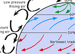

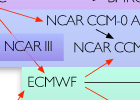

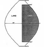

|
| How modules for features of the climate system were incorporated one by one into models, 1970s-2000s. (If the figure were extended to the 2020s it would show an additional module calculating the dynamics of large ice sheets.) — Source: IPCC report (2001a), Technical Summary, Box 3, Fig. 1, p. 48. For a later, more complete version see Donner et al. (2011), p. 36. |
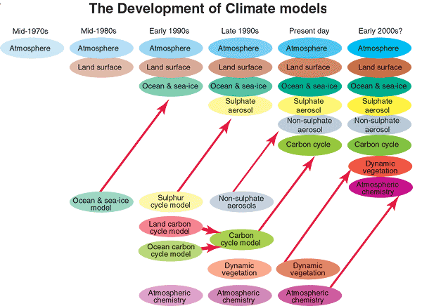
Weather prediction had meanwhile advanced along its separate path. Meteorologists had their own approximations, shortcuts that would wreck a model that ran for a virtual month. Meteorologists didn't care since their predictions wandered chaotically away from real weather within a week or two anyway. Climate modelers had to stick closer to real physics. With the ceaseless improvement of atmospheric data, software techniques, and supercomputer hardware, some teams began working toward unified models. Already in the mid 1980s, when a new generation of supercomputers forced teams to rewrite much of their code from scratch, programmers began to look over one another's shoulders. By the 1990s the U.K. Meteorological Office was sharing some atmospheric physics code between its weather and climate models. |
||
| In the late 2010s integration of the Met Office models was virtually complete, while other teams were working toward the same goal. In a one-hour run of their unified model the Met Office could simulate current global weather accurately enough for daily short-term weather predictions, and with the identical set of equations and parameters (plus code for slowly-changing features like ice sheets) they could do weeks-long runs to calculate climate into the next century.(102b) | ||
| For projecting the future climate, experts still had plenty of work to do. The range of modelers' predictions of global warming for a doubling of CO2 remained broad, anywhere between roughly 1.5 and 4.5°C. The ineradicable uncertainty was still caused largely by ignorance of what would happen to clouds as the world warmed. Much was still unknown about how aerosols helped to form clouds, what kinds of clouds would form, and how the various kinds of clouds would interact with radiation. That problem came to the fore in 1995, when a controversy was triggered by studies suggesting that clouds absorbed much more radiation than modelers had thought. Through the preceding decade, modelers had adjusted their calculations to remove certain anomalies in the data, on the assumption that the data were unreliable. Now careful measurement programs indicated that the anomalies could not be dismissed so easily. As one participant in the controversy warned, "both theory and observation of the absorption of solar radiation in clouds are still fraught with uncertainties."(102c) |
|
|
| Incalculable and Calculable Risks TOP OF PAGE | ||
| The rapidly changing architecture of supercomputers, in particular the advent of massively parallel computing in the 1990s, forced each team to repeatedly revise its codes and even their basic computational methods. By now each of the big models embodied the life work of hundreds of scientists and software developers. | ||
| As the 21st century began, one of the biggest problems was subtleties in the physics of clouds that might significantly affect the models' predictions. To take just one example, the most respected critic of global warming models, Richard Lindzen, started a long debate by speculating that as the oceans warmed, tropical clouds would become more numerous. They would reflect more sunlight, he said, making for a self-stabilizing system.(103) And in fact the models and observations were still so imprecise that experts could not say whether changes in cloudiness with warming would tend to hold back further global warming, or hasten it by trapping radiation rising from below, or have little effect one way or the other. Despite these uncertainties, the effects of clouds did seem to be pinned down well enough to show that they would not prevent global warming. Indeed climate experts (aside from Lindzen and a bare handful of other experts) were now nearly certain that serious global warming was visibly underway. Still, difficulties with calculating clouds remained the main reason that different GCMs gave different estimates for the warming in the late 21st century. The projections ranged from only a degree or two Celsius to half a dozen degrees, and into the 2020s the modelers were unable to narrow the range.(104) |
|
|
| It was also disturbing that model calculations did not seem to match observations of the temperature structure of the atmosphere. In 1990 Roy Spencer and John R. Christy of the University of Alabama, Huntsville had published a paper that eventually resulted in hundreds of publications by many groups. Although warming might be observed at the Earth's surface, they pointed out that satellite measurements showed essentially no warming in recent decades at middle levels of the atmosphere — the upper troposphere. More direct measurements by balloons and radiosondes (rockets) likewise showed no warming there. However, a greenhouse-warming "tropospheric hot spot," especially in the tropics, had been predicted by all models clear back to the 1975 work of Manabe and Wetherald.(104a) Indeed not only greenhouse warming, but anything that produced surface warming in the tropics should also warm the atmosphere above it, through convection. People who insisted that global warming was a myth seized on this discrepancy. They said it proved that people should disbelieve the computer models and indeed all expert opinion on global warming. But was it the models that were wrong, or the data? |
|
|
| The satellites, balloons, and radiosondes that measured upper atmosphere temperatures had been designed to produce data for daily weather prediction, not gradual long-term climate changes. Over the decades there had been many changes in practices and instrumentation. A few meteorologists buckled down to more rigorous inspection of the data, and gradually concluded that the numbers were not trustworthy enough to disprove the models. The orbits of the satellites, for example, had shifted gradually over time, introducing spurious trends. As more groups weighed in, the 1990s were full of controversy and confusion. Some groups manufactured adjustments to the data that did show upper-troposphere warming; Spencer and Christy adjusted their own data and stoutly maintained their distrust of any form of global warming. The problem was resolved in 2004-2005, when different groups described errors in the analysis of observations. For example, the observers had not taken proper account of how instruments in the balloons heated up when struck by sunlight. The mid-level atmosphere had indeed been warming up. Even Spencer and Christy conceded that they had made mistakes.(105) | ||
| It was one more case, like the CLIMAP controversy, where computer modelers had been unable to tweak their models until they matched data, not because the models were bad but because the observations were wrong. In this case the raw data were fine, but numbers are meaningless until they are processed; it was the complex analysis of the data that had gone astray. (In the public sphere, even a decade later Christy and others would continue to rely on the slippery satellite data to deny that the world was warming. With enough types of observations, it is usually possible to select some that will support any position.)(105a*) | ||
| More important, the high stratosphere was undoubtedly getting cooler. This was what modelers had predicted ever since Manabe and Wetherald's pioneering 1967 paper showed — an inevitable effect of the increase of greenhouse gases blocking radiation from below. A stratospheric cooling would not arise from other forces that could warm the surface. Increased solar radiation, for example, should produce warming at all levels. The stratospheric cooling was one component of the greenhouse effect "signature" that impressed the IPCC in 2001 and thereafter | ||
| The skeptics were not satisfied, for some discrepancies remained. In particular, the modelers still could not reproduce some observations of temperature trends in the upper troposphere in the tropics. Exhaustive reviews concluded that there was room for the discrepancies to eventually be resolved, as so often before. It might be the models that would be adjusted. More likely the observations, still full of uncertainties and spanning only a couple of decades, would again turn out to be less reliable than the models. And so it proved. In 2008 a group reported, "there is no longer a serious discrepancy between modeled and observed trends."(105b) |
|
|
| The models were now quite good at reconstructing the average global climate and projecting how it would change over at least the next several decades. However, the chaotic nature of the climate system prevented such accuracy for relatively small regions like, say, the United States or Western Europe. If you did multiple runs starting with slightly different initial conditions, each run would get a similar global average but quite different regional changes over the decades. Even averaging over a set of models you could come up with substantially more warming for one of these regions than actually happened, or less. | ||
| Critics kept focusing on such minor discrepancies and pointing them out as publicly as possible. Usually this was an exercise in "cherry-picking," pouncing on the few items among many hundreds that supported a preconceived viewpoint. Yet modelers readily admitted that many uncertain assumptions lurked in their equations. And nobody denied the uncertainties in the basic physical data that the models relied on, plus further uncertainties in the way the data were manipulated to fit things together | ||
| Modelers were particularly worried by a persistent failure to work up a reasonable simulation of the climate of the mid-Pliocene epoch a few million years ago, when CO2 and global temperatures had reached levels as high as those predicted for the late 21st century. Paleontologists claimed that the Pliocene had seen only a modest difference in temperature between the poles (much hotter than now) and the equator (not much hotter). The modelers could not figure out how the oceans or atmosphere could have moved so much heat from the tropics to the poles. A paleontology team warned in 2018 that something was missing, so that "climate projections may underestimate long-term warming... by as much as a factor of two. | ||
| A giant collaboration among 16 computer teams came together to study this analog of our possible future, and by 2020 they were able to roughly reproduce the hot Arctic and other features of the era, although for some regions the calculations still did not match the geological data. Modelers had also struggled with the Paleocene-Eocene Thermal Maximum (PETM) 56 million years ago, when the North Pole had suddenly become incredibly hot; here too by 2020 some models managed to reproduce the gross global features. Some experts nevertheless continued to worry that the unusually warm poles at that time might point to something important missing from the models. | ||
| The problem was worse for the Cretaceous epoch — a super-greenhouse period a hundred million years ago when the Earth had a CO2 level several times higher than at present. Paleontologists reported dinosaurs in Alaska, basking in warmth not much cooler than the tropics. No model had managed to reproduce that. If our greenhouse emissions heated Earth that far, there might be conditions (radical changes in cloudiness? in ocean circulation? undreamt-of feedbacks?) stranger than anything the models were designed to calculate.(106*) | ||
| For a climate not greatly unlike the present, however, all the significant mechanisms must have gotten incorporated somehow into the parameters. For the models did produce reasonable climate patterns for such different conditions as summer and winter, the effects of volcanic eruptions, substantially colder and warmer past geological periods, and so forth. At worst, the models were somehow all getting right results for wrong reasons — flaws that would only show up after greenhouse gases pushed the climate beyond any conditions that the models were designed to reproduce. If there were such deep-set flaws, that did not mean, as some critics implied, that there was no need to worry about global warming. If the models were faulty, the future climate changes could be worse than they predicted, not better. |
|
|
| Those who still denied there was a serious risk of climate change could not reasonably dismiss computer modeling in general. That would throw away much of the past few decades’ work in many fields of science and engineering, and even key business practices. The challenge to them was to produce a simulation that did not show global warming. Now that personal computers were far more powerful than the most expensive computers of earlier decades, it was possible to explore thousands of combinations of parameters. But no matter how people fiddled with climate models, whether simple one- or two-dimensional models or full-scale GCMs, the answer was the same. If your model could simulate something at all resembling the present climate, and then you added some greenhouse gases, the model would show significant global warming.(107) |
|
|
| The modelers had reached a point where they could confidently declare what was reasonably likely to happen. They did not claim they would ever be able to say what would certainly happen. Different model runs continued to offer a range of possible future temperatures, from mildly bad to disastrous. Worse, the various GCMs stubbornly continued to give a wide range of predictions for particular regions. Some things looked quite certain, like especially strong warming in the Arctic (hardly a prediction now, for such warming was becoming blatantly visible in the weather data). Most models projected crippling heat and dryness in the American Southwest and Southern Europe. But for many of the Earth's populated places, the models could not reliably tell the local governments whether to brace themselves for more droughts, more floods, or neither or both. |
|
|
| By the dawn of the 21st century, climate models had become a crucial source of information for policy-makers and the public. Where once the modelers had expected only to give talks at small meetings of their peers followed by formal publication in obscure scientific journals, their attention now focused on working up results to be incorporated in the reports that the IPCC issued to the world's governments. Struggling to provide a better picture of the coming climate changes, the community of modelers expanded and reorganized. | ||
| As ever more modeling groups joined in, they wanted to systematically compare and evaluate their products. During the 1990s most of the world's computer teams collaborated in an international Atmospheric Model Intercomparison Project. Each team ran its model with the same initial numbers for sea surface temperatures and on the same computer (at the Livermore lab), aiming not so much to rank the quality of their models as to identify their individual strengths and weaknesses. The exercise was so useful that in 1996, even before the atmospheric models project published its formal report, the modeling community launched a Coupled Model Intercomparison Project (CMIP) incorporating the oceans as well as the atmosphere. It was the first of a series of CMIPs that would become a central ongoing activity, forcing the groups to agree on schemes for representing features of climate and formats for reporting their data. |
|
|
| That was not as simple as it might seem. Just to make sure "that the words used by each group and for each model have the same meaning," a French team leader remarked, "requires a great number of meetings." But once all the numbers were given a well-defined meaning, the computer outputs could serve as raw material for groups that had nothing to do with the originators. That opened new paths for criticism and experimentation. A joint archive was established, which already by 2007 contained more than 30 terabytes of data utilized by more than 1000 scientists. Groups were exchanging so much data that it would have taken years to transfer it on the internet, and they took to shipping it on terabyte hard drives.(108) |
|
|
| There were about a dozen major teams now and a dozen more that could make significant contributions. The decades of work by teams of specialists, backed up by immense improvements in computers and data, had gradually built up confidence in the prediction of global warming. It was largely thanks to their work that, as the editor of Science magazine announced in 2001, a "consensus as strong as the one that has developed around this topic is rare in the history of science."(109*) |
<=>Aerosols |
|
| Each computer modeling group normally worked in a cycle. When their model began to look outdated, and still more if they managed to acquire a new supercomputer, they would go back to basics and spend a few years developing a new model. It was no simple task. The laborious tuning of parameters to produce a realistic final climate meant that a small error in the way the old model had calculated a process might have been compensated by small errors in other processes. Introducing a minor new wrinkle (for example, a better way to calculate convection in the tropics) often introduced unexpected feedback that made the entire model crash. Once a team had persuaded their model to produce stable results that looked like the real world, they would spend the next year or two using it to analyze climate processes, gathering ideas for the next cycle. | ||
| After finishing their part of the IPCC's 2001 report, the modeling community worked to synchronize the teams' separate cycles. By early 2004, nearly all the major models simultaneously reached the analysis stage. That made it possible for the teams to share and compare data in time to produce results for the next IPCC report, scheduled for 2007. In the end 17 groups contributed, up from four for the first IPCC report. They got funds from their individual national authorities or simply put in personal time alongside other projects (successful scientists work far beyond a 40-hour week). Their models were dramatically better than those of a decade earlier. The average model now had impressive "skill" (as modelers termed it) in representing the world's observed winds, rains, and so forth, and the average over the entire set of models was more accurate still.(110) | ||
| The IPCC pressed the teams to work out a consensus on a specific range of possibilities for publication in the 2007 report. CMIP3 broke new ground by running each of its models with a range of different scenarios for the rate of global emissions, to see what these might mean for future climate. The work was grueling. After a group had invested so much of their time, energy, and careers in their model, they could become reluctant to admit its shortcomings to outsiders and perhaps even to themselves. A frequent result was "prolonged and acrimonious fights in which model developers defended their models and engaged in serious conflicts with colleagues" over whose approach was best.(111) Yet in the end they found common ground, working out a few numbers that all agreed were plausible. |
|
|
| The most likely number for climate sensitivity had scarcely changed since the pioneering computer estimates of the 1970s. Doubling the level of CO2, which was expected to come well before the end of the 21st century, would most likely bring a rise of roughly 3°C in the average global temperature. (This was the "Charney sensitivity," looking ahead no more than a century.) The uncertainty also remained as before: the number might be as low as two degrees, or as high as five or six. The next half-dozen years of work failed to advance this. Changes in cloudiness, including the complicated effects of aerosol pollution on clouds, continued to be the largest source of uncertainty. "We're just fine-tuning things," a leading modeler remarked in 2012. "I don't think much has changed over the last decade."(112) |
|
|
| The modelers' sensitivity estimate got an entirely independent confirmation in the geologists' latest observations for how global temperatures had connected with the level of CO2 in the past. By now ingenious studies had produced estimates for both CO2 and temperature in a dozen eras from recent to the very distant. One example was a 1987 discovery that the density of microscopic pores in leaves (stomata) had sharply decreased during the 20th century. The decrease was in proportion to the rise of CO2 in the air — plants were adjusting to the higher gas level. Thus fossil leaves of similar species (magnolia, for one) could be used as gauges of ancient CO2 levels. For example, a 1999 study of fossil plants from the end of the Triassic period, one of the worst extinction events in Earth history, reported highly elevated CO2 along with deadly global heating. |
|
|
| Taken all together, the evidence indicated that a doubling of CO2 would not warm the planet less than 1.5°C. The upper limit was harder
to fix, since doubled CO2 would push the atmosphere
into a state not seen for tens of millions of years. The models could
not reliably calculate such a foreign condition, and the geological evidence
for temperatures and gas levels so long ago was hard to interpret. In the end
the geologists and the computer modelers independently concluded that
doubling CO2 was scarcely likely to bring a long-term rise
greater than 5°C averaged over the entire planet. That was scant comfort: a rise of that magnitude would bring global changes unprecedented in the experience of the human race. Nor was anyone confident that emissions could be stopped by the time the level had doubled.(113*) |
Projected temperatures for 2080-2099 (rise above the 1980-1999 level, mean of multiple GCMs) for the "A2" scenario, in which the world begins now to restrict its greenhouse gas emissions. |
|
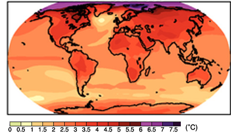
|
What if the scientists were too optimistic about their level of certainty? A minority of experts were beginning to worry that the IPCC reports did not give humanity proper warning. It was all very well to hammer out a conservative consensus on what climate changes were most likely. But shouldn't we consider not just what was most likely, but also the worst things that might in fact happen? What if aerosol and cloud processes were a bit different from what the models assumed, although still within the range of what physics allowed? After all, these parameters could still not be pinned down from first principles, but had to be laboriously adjusted for each model; without this "tuning" no model could realistically reproduce even the present climate. Confirming such worries, a group reported in 2008 that smoky "black carbon" emissions had a much stronger effect than the models had guessed, making for worse warming. And what if any of the many amplifying feedbacks turned out to be stronger than the models estimated, once regions warmed into a condition for which we had no data? Several new studies pointed in that direction. The probability that the IPCC had seriously under-estimated the danger seemed easily as great as one in ten — far above many risks that sensible people normally took precautions against.(113a) |
<=Aerosols |
| A comprehensive study that ran models with 400 different combinations of likely parameters announced in 2009 that the IPCC had cautiously underestimated a great deal. In the worst case — where humanity kept heedlessly burning ever more fossil fuels to the end of the century — it was even odds that the world would see a 5°C rise. If the average global temperature did soar that high, it would launch the planet into a state utterly unlike anything in the history of the human race (even a 2°C rise would go above anything known since the spread of agriculture). And still higher temperatures were entirely possible.(114) |
|
| The computer modeling teams now launched an even more massive cooperative multi-year effort, CMIP5, completing most of the work by 2013 in time to guide the IPCC's 5th report. (Meanwhile, planning for CMIP6 was already underway; by 2018 it would embrace 33 modeling groups in 16 countries). The scale and level of organization was beyond anything in other sciences. Each major family of models was tended in its own national institute, housed in a large modern building where hundreds of workers continually revised, expanded and tested their software. Each institute was in daily communication with its peers, exchanging visits, data, code, and boisterous arguments. The growth of the climate modeling enterprise over a short half century had been fabulous, as if a little inn at a crossroads had burgeoned into a bustling city. | |
| For all the effort, the results of the intercomparison projects of the 2010s were scarcely different from earlier attempts. "The drive to complexity has not reduced key uncertainties," two of the experts admitted. "Rather than reducing biases stemming from an inadequate representation of basic processes, additional complexity has multiplied the ways in which these biases introduce uncertainties in climate simulations." The IPCC reported in 2014 that equilibrium sensitivity for doubled CO2 was "likely" to be in the range 1.5 to 4.5°C — exactly the same numbers the Charney Panel reached 34 years earlier, albeit now with higher confidence and on a firmer foundation of evidence.(115*) | |
| If we managed to halt emissions at the doubled CO2 level, would the global temperature rise immediately halt? The Charney Panel and other early studies had warned that if we cut back our emissions, warming would continue for decades until the oceans reached an equilibrium.(see above). However, the pioneering calculations could not attempt to follow all the complexities of the evolving geochemical carbon cycle. The early computer modelers had put in a "step function," a simple one-time doubling of the CO2 level as if a planet-load of the gas was abruptly dumped into the atmosphere. A different picture emerged once computers became powerful enough to track how the level would actually change year by year as emissions were wrestled down. Since the oceans and plants would meanwhile be absorbing CO2 from the atmosphere, it seemed that global temperature would stabilize almost at once when net emissions got to zero. This was explained around 2010, but nearly a decade passed before journalists alerted the entire scientific community, to say nothing of the public, to the good news that cutting emissions was likely to bring an immediate reward, To be sure, that would only be true if we stopped before temperatures got high enough to pass some critical threshold for a process that would set in motion irreversible further heating.(115a*) |
|
| That was the short-term answer. Full equilibrium would only be reached after centuries of melting ice fields and changes in forest cover, tundra, ocean circulation, and other processes that even the newest models scarcely understood. And by that time the world would be warmer, different in obscure ways from the present. Some studies of ancient climates indicated that, unfortunately, sensitivity would probably be higher in a warmer world. | |
| A striking illustration of the models' shortcomings came in a widely noted 2016 paper by Ivy Tan, a graduate student at Yale University. Looking at data accumulated by a satellite launched ten years earlier, she analyzed the fraction of ice crystals in one common type of cloud and found that the clouds held less ice than modelers supposed. The modelers had worked with parameters for an average mixture of supercooled droplets and ice crystals, but real clouds were a jumble of clumps with different properties. When a team plugged the correction into their climate model they saw the equilibrium sensitivity jump up by a full degree. When other experts were asked for their opinion they could only shrug — yes, all the models would need more work before they could provide solid long-term projections. | |
| Satellites deployed over the southern oceans in 2014-2017 also showed that the effects of aerosols on cloud formation ("susceptibility"), and thus on cooling the planet, were considerably stronger than theorists had estimated. That explained why some computer modeling teams had resorted to artificially tuning aerosol interactions in order to reproduce the actual global temperature record (they had assumed they were compensating for some unknown aerosol warming mechanism).(116) |
|
| Different modeling teams always got somewhat different results. There were many reasons for the variations; models even diverged in basic calculations of the effect of CO2 on infrared radiation. But the biggest source of uncertainty remained the behavior of clouds, and in particular how the aerosols that humanity was emitting affected clouds. One major impediment was a gross absence of global data. Modelers could only guess at how aerosol emissions had risen, or perhaps declined, in different regions over the decades, and the uncertainty seeped into the work of testing and adjusting models against the historical record of climate changes. Technical problems and politics delayed the launch of a satellite that could measure aerosols until 2024. | |
| Hundreds of experts were now devoting their careers to making marginal improvements in the models. For example, in 2017 the authors of the widely used Community Earth System Model worked up a more elaborate version, and found it over-estimated the cooling effects of the sulfate pollution that had spread in the mid 20th century. Development was held up for half a year for exhaustive discussions between specialists in cloud-aerosol parameters and specialists in emissions data. In the end both sides had to make revisions. This was just one of many examples of grueling cooperative work by multiple teams, adjusting parameters to get a better reproduction of actual weather patterns. | |
| A particularly galling discrepancy was so persistent that it got its own name, the "double ITCZ problem." Our actual Earth has a band of rainstorms north of the Equator in the Pacific Ocean, which meteorologists style the Intertropical Convergence Zone (ITCZ). In many state-of-the-art computer models a second, spurious band showed up south of the Equator. "This double ITCZ problem," one expert lamented in 2019, "has plagued generations of GCMs for more than two decades." | |
| Similarly troubling was the "cold tongue," an anomaly that in 2023 one expert called "the most important unanswered question in climate science." A swath of relatively chilly water was observed in the Pacific Ocean off of South America where most climate models calculated the water should be getting warmer. The discrepancy, first pointed out in 1997, presumably reflected significant complexities that climate models had not incorporated. If the cold persisted in future decades, global warming might come rather slower than most models projected.(117) | |
| Yet another problem, perhaps more fundamental, came to light in attempts to compute the climate of the middle Miocene period some 15 million years ago. Measurements of the CO2 level back then with ingenious chemical techniques and other methods found a level roughly as high as we would get by 2100, unless nations clamped down hard on emissions, and the average temperature had been an astonishing 7°C warmer than our pre-industrial climate. Models could not reproduce this. An expert asked, “are positive feedbacks missing in the models?” Some geologists, however, thought that Miocene CO2 levels had actually been much higher, perhaps due to natural volcanic processes. Whatever happened back then, it was troubling to think that an unexpected and fatal feedback loop might kick in at some point as we kept perturbing the planet.(117a) | |
| On the other hand, simulations were pretty good for most features of the recent climate, and of past climates that were not radically different. For example, satellite observations of the distribution of clouds around the globe showed that changes since the 1980s as CO2 rose resembled what mainstream models had calculated — "the cloud changes most consistently predicted by global climate models are currently occurring in nature." | |
| That was just one of many demonstrations that the models had real predictive power. Another example was the "Holocene temperature conundrum." Global temperature data from fossils buried in sea-sediment cores showed a gradual temperature decline since the warm mid-Holocene period 8,000 years ago. But when modelers in the 2010s tried to reproduce this, try as they might they got a slight warming instead. The discrepancy was resolved by studies of fossil pollen in lake beds. The error turned out to lie in the analysis of the pollen data; the models' prediction (or "retrodiction") was correct. Once again the fact that models could not be twisted to get a wrong result argued that they were somehow in touch with reality. Modelers and paleontologists interested in the much hotter Miocene period collaborated to see whether their problem too was in wrong estimates of past conditions, or whether the models failed when the planet heated past some point | |
| For climates not grossly unlike our own, the models looked trustworthy. You could set the observed temperature record against the projections that modelers had made as far back as the 1980s. Critics made much of the way some of the early projections turned out to have calculated a bit less warming, or a bit more warming, than actually happened over following decades. In fact the discrepancies were mainly because the modelers had not correctly guessed the amount of pollution and greenhouse gases that civilization would produce over the years. If the actual emissions were taken into account, nearly every model had done well. They had given fair warning of how the planet would heat up in response to our emissions.(118) | |
| The future was another matter. We were pushing the planet into a condition for which the past provided little data. When modeling teams got together in Barcelona in 2019 to work out mutual problems ahead of submitting their results for the next IPCC report, they reached some uncomfortable conclusions. For the first time the models agreed on a lower limit for warming with doubled CO2. We would not be saved by the good luck of a sensitivity below 2°C. At the other extreme, the results were less certain and even more disturbing. The most advanced supercomputers, incorporating improved understanding and more complex calculations for cloud feedbacks, aerosol susceptibility, and other influences, now found an upper limit of sensitivity approaching 5°C. Some calculations got even more frightening numbers. | |
| However, the last ice age and more distant geological eras had generally not shown such high sensitivity. And for the past few decades, where the temperatures and CO2 rise were known precisely, the models that had high sensitivity calculated greater warming than had actually happened. Taking all the climate models together, the actual temperature rise had been near the lower bound of the range of projections. Something had to be amiss in the models. | |
| Researchers rounded up the usual suspects — cloud processes. Comparing model results with satellite observations turned up discrepancies. In particular, when tropical clouds in the "hot" models got warmer, they rained out and vanished more rapidly than actual observed clouds. Thus the simulated cloudiness had less cooling effect than real clouds. Presumably other features in the "hot" models also needed a closer look (for one, the perennially problematic aerosols). All this brought "a collective sigh of relief" from the modelers. Better to have labored for half a dozen years producing flawed results than face a high risk of apocalyptic climate change! | |
| In its 2021 report the IPCC at long last managed to set limits on sensitivity tighter than the 1.5–4.5°C estimate that had ruled ever since 1979. Now the "likely" (that is, 67% probability) range was given as 2.5–4°C, abandoning hopes that doubling CO2 might have only mild consequences. The "best estimate" for sensitivity was still 3°C. To get reliable numbers, the panel had given greater weight to the computer models that were best at reproducing the warming trend of the past century (a test the "hot" models mostly failed). | |
| With progress in computer models seemingly stalled, for this report the IPCC expanded its field of view. They now used the models' outputs as only one factor in the sensitivity estimate. Over the decades paleontologists had been developing ever more ingenious and precise ways to measure both the level of CO2 and the temperature in past geological eras—not only the recent ice ages but back to the era of the dinosaurs and even farther back. Their findings were now reliable enough to provide a second, wholly independent approach to calculating sensitivity. In long discussions (mostly online, with the COVID-19 pandemic restricting travel) the scientists found they could add a third independent approach. There was now more than half a century of good data on rising global temperatures and rising CO2 levels, allowing new kinds of analysis that reinforced the other two. |
|
| To be sure, the problems with clouds showed that future research might bring more surprises, and the model projections stubbornly differed in many respects. For example, the effects of aerosols on clouds were so difficult to either observe or calculate precisely that modelers tended to simply adjust parameters until the model results looked plausible. That left room for wide variations (and raised a risk that the long-standing "most likely" 3°C sensitivity could become a self-reinforcing assumption). If the cooling effect of pollution had been underestimated, sensitivity might be seriously higher than the IPCC's best guess. The realization that the fearfully "hot" computer models with their high upper temperature ranges were flawed did not prove that the more temperate models were flawless; it pointed to persistent uncertainty.(119) |
<=>Impacts <=>Aerosols |
| Worries sharpened in the next few years. A modest El Niño in 2023-24 boosted the global temperature in a stunning jump, well beyond what models had anticipated. One cause showed up in satellite measurements of the sunlight reflected from Earth; analysis found that in recent decades the planet had been reflecting less and less of the sunlight falling on it. The imbalance between the solar energy coming in and the heat energy radiated out had accelerated, doubling since the start of the century (it was now a bit above 1 watt per square meter — as if a 100-watt light bulb was burning above every ten by ten meter square of Earth's surface). No wonder, then that the rate of global temperature rise in the decade 2015-2025 was much higher than the rate that had prevailed earlier. | |
| One reason for the decline in reflectivity was quickly recognized: decreasing cloudiness. That might relate to the stubborn uncertainties in the effects of aerosols — some of the decrease was in regions where pollution controls had tightened. But it might also be a self-sustaining effect of global warming itself. Some of the planet’s decreased reflectivity came from shifts in low-level clouds and storms in tropical and mid latitudes, shifts that suggested the entire general circulation of the atmosphere was readjusting. All of this seemed incompatible with global models that exhibited low sensitivity. | |
| Aerosols and clouds were not the only weak points in the models. For example, a 2024 study showed that the numbers that all models had used for decades to describe the annual uptake of CO2 by plants had seriously underestimated the actual uptake. That put in question calculations of, among other things, the climate effects of drought and deforestation. Meanwhile the reassurance provided by paleontological data was called into question by studies that reported unexpectedly high sensitivity in some past eras. | |
| The IPCC itself had warned that the high-sensitivity models were examples of "tail risk," providing "insights into low-likelihood, high-impact outcomes, which cannot be excluded based on currently available evidence." Formally, beyond the “likely” range of sensitivity the IPCC gave a "very likely" (at least 90% probability) range of 2–5°C. — which meant a real risk that the number could even be above 5°C. The differences were between a future that was bad, or very bad, or appalling.(120) | |
| If the future was murky, models were bringing the deteriorating climate of the present into sharper focus. Since the early 2000s a few teams had taken up a new question: was global warming responsible for the weather disasters that seemed to be multiplying? While models differed in details of their predictions, they gave broadly similar answers when asked to compare two extreme cases: a world where humans had never emitted any greenhouse gases, and our actual 21st-century world. They found that many of the worst recent floods, heat waves, and droughts would have been less severe in the no-emissions world. For example, a 2017 study resolved uncertainties in the long-standing prediction that land in middle latitudes would get drier. The drying was already observable and was "mainly attributable" to the human influence on climate.(121) Ever more of these "attribution" studies showed that human emissions not only would bring harm, but were already undeniably harming agriculture, human health, and natural ecosystems. The annual costs were rising into many billions of dollars, the annual deaths were unequivocally in the thousands and arguably a hundred times that. Attribution of specific events became a new frontier of computer work. |
<=Impacts |
| Studies of likely future impacts in particular regions took an increasing share of computer time, driven by demands from policy-makers who were struggling to plan how their communities should prepare. Climatology was returning to its roots a century back, when agencies had confidently issued calculations of 100-year floods and the like based on the statistics of past decades. Now the rise of greenhouse gases had detached the future from the past. And no matter how good the enormous computer models were for projecting global averages, they were baffled when it came to rare extreme events like terrible heat waves and droughts. Different models and even different runs of the same model could give divergent answers, and sometimes all of the models turned out to be wrong. The modeling community, a member admitted in 2023, is "not yet ready to provide society with robust and actionable information." The current models, another expert lamented, "can't even determine whether some places will experience more droughts or floods, whether governments should build reservoirs or levees."(122) | |
| For all the millions of hours the modelers had devoted to their computations, in the end they could not say exactly what climate change would be like in a given place. But for the planet and our civilization as a whole, they could say with confidence that our emissions were already doing serious harm, that the harm would get worse, and that unless strenuous measures were taken without delay we faced a grave risk of global catastrophe.
What do the current models predict global warming will mean for
humanity in practical terms? See the summary of expected Impacts of Climate Change. |
|
Home
Simple Models of Climate
Ocean Currents and Climate
Aerosol Hazes
Supplements:
Basic Radiation Calculations
Arakawa's Computation Device
Chaos in the Atmosphere
Reflections on the Scientific Process
| NOTES |
1. The first, much shorter version of this essay was partly based, by permission, on Edwards (2000b). For a complete history of climate modeling see Edwards (2010), Easterbrook (2023), and (especially for technical developments) Donner et al. (2011) and Randall et al. (2018). BACK
2. Simpson (1929b), p. 74. BACK
3. For the history of work on the general circulation, see Lorenz (1967), 59ff. BACK
4. Nebeker (1995); for Bjerknes and scientific meteorology, see also Friedman (1989). BACK
5. Richardson (1922), forecast-factory p. 219, "dream" p. ix; see Nebeker (1995), ch. 6, esp. pp. 81-82; Lynch (2006). BACK
6. Bolin (1952), p. 107. BACK
7. Here and below: Aspray (1990); Nebeker (1995), ch. 10. For a comprehensive study published after the bulk of this essay was written, see Harper (2008). BACK
8. Charney (1949); for a comprehensive discussion, Charney and Eliassen (1949); the first experiment (raising up the Himalayas) in a GCM was Mintz (1965). BACK
9. Charney (1949), pp. 371-72; for general discussion of heuristic modeling (including Charney's filtering), see Dalmedico (2001). BACK
10. An example of important mathematical work is Phillips (1951); for all this history, see Nebeker (1995), pp. 87, 141-51, 183; Smagorinsky (1983); also Smagorinsky (1972); Kutzbach (1996), pp. 362-68. BACK
11. Charney et al. (1950), quote p. 245; Platzman (1979). See Archer and Pierrehumbert (2011), pp. 78-80. BACK
13. Bergthorsson et al. (1955). BACK
14. For operational forecasting, see also Cressman (1996). BACK
15. Phillips (1956); on dishpans, see also Norman Phillips, interview by T. Hollingsworth, W. Washington, J. Tribbia and A. Kasahara, Oct. 1989, p. 32, copies at National Center for Atmospheric Research, Boulder, CO, and AIP. See also quote by Phillips in Lewis (2000), p. 104, and see ibid. passim for a detailed discussion of this work; "Classic": Smagorinsky (1963), p. 100; already in 1958 Mintz called it a "landmark," see Arakawa (2000), pp. 7-8. BACK
16. Conference: Pfeffer (1960); Smagorinsky (1983); Lewis (2008), Smagorinsky quote: p. 1344.. BACK
17. Manabe et al. (1965); it was "the first model bearing a strong resemblance to today's atmospheric models" according to Mahlman (1998), p. 89; see also Smagorinsky (1963), quote p. 151; Smagorinsky et al. (1965). See also Manabe and Broccoli (2020); Manabe, interview by P. Edwards, March 14, 1998, AIP, online here. BACK
18. Arakawa et al. (1994). BACK
19. Johnson and Arakawa (1996), pp. 3216-18. BACK
20. The oceans were given an infinite heat capacity (fixed temperature), while land and ice had zero capacity. Mintz (1965) (done with Arakawa); this is reprinted in Bates et al. (1993); see Lorenz (1967), p. 133; Arakawa (1970); Edwards (2010), p. 158. BACK
21. Arakawa and Schubert (1974) was a major step, and briefly reviews the history. Blinking: Edwards (2010), p. 340. BACK
22. Norman Phillips, interview by T. Hollingsworth, W. Washington, J. Tribbia, and A. Kasahara, Oct. 1989, p. 23, copies at National Center for Atmospheric Research, Boulder, CO, and AIP. BACK
W. Washington photo by UCAR, Ginger Hein, CC BY-NC 4.0, via OpenSky BACK
23. Kasahara and Washington (1967); Edwards (2000b). For Leith and early models in general see Easterbrook (2023), ch.6. BACK
24. National Academy of Sciences (1966), vol. 2, pp. 65-67. BACK
25. Lorenz (1967), pp. 26, 33, 90-91, ch. 5 passim. BACK
26. Smagorinsky (1970), p. 33 (speaking at a 1969 conference); similarly, see Smagorinsky (1972), p. 21; "future computer needs will be tempered by the degree to which... we can satisfy the requirements for global data." National Academy of Sciences (1966), vol. 2, p. 68; Wilson and Matthews (1971), p. 112-13. BACK
27. Lorenz (1967), quote p. 10; "As for a satisfactory explanation of the general circulation... none exists": Rumney (1968), p. 63. BACK
28. Lorenz (1967), p. 8, see pp. 134-35, 145, 151. BACK
29. Kellogg and Schneider (1974), p. 1166. BACK
30. See the "pyramid" typology of models developed in Shine and Henderson-Sellers (1983); McGuffie and Henderson-Sellers (1997), pp. 44, 55 and passim; Adem (1965); Green (1970). BACK
31. A.R. Robinson (about ocean modeling) in Reid et al. (1975), p. 356. BACK
32. "The use of mathematical computer models of the atmosphere is indispensable in achieving a satisfactory understanding..." Matthews et al. (1971), p. 49; a followup study the next year, gathering together the world's leading climate experts, likewise endorsed research with GCMs. Wilson and Matthews (1971). The section on GCMs was drafted by Manabe. BACK
33. Nebeker (1995), p. 179. BACK
34. Edwards (2000); Edwards (2010); Nebeker (1995), p. 176. BACK
35. A more fundamental problem of detail was parameters for the absorption and scattering of solar radiation by clouds, aerosol particles, etc. Lacis and Hansen (1974); Hansen et al. (1983); Hansen, interview by Weart, Oct. 2000, AIP, and Hansen et al. (2000), pp. 128-29. BACK
36. Spectral methods: Bourke (1974), Easterbrook (2023), p. 141; see Edwards (2000), p. 80 gives references to 1970. Cubed sphere: Putman and Lin (2007), see Geophysical Fluid Dynamics Laboratory, Princeton, "HiRAM (HIgh Resolution Atmospheric Model)", online here. BACK
37. For more see Edwards (2000), Edwards (2010). BACK
38. Mintz (1965), p. 153. BACK
39. He recalled that the committee meetings prompted him to ask Manabe to add CO2 to his radiation model. Smagorinsky, interview by Weart, March 1989, AIP. National Academy of Sciences (1966). BACK
41. Manabe and Strickler (1964). For all this see Manabe, interview by Paul Edwards, March 15, 1998, AIP. BACK
42. E.g., Arrhenius (1896) (who also calculated for increases by factors of 1.5, 2.5, and 3 as well as lowered levels); Plass (1956); Möller (1963). BACK
43. Manabe, interview by P. Edwards, March 14, 1998, AIP, online here. Manabe and Wetherald (1967). On Manabe see Will (2021) and for full history of his models, Manabe (2019), Manabe and Broccoli (2020) , Randall et al. (2018) }. BACK
44. Broecker, interview by Weart, Nov. 1997, AIP; Forster (2017); Roz Pidcock, "The Most Influential Climate Change Papers of All Time," CarbonBrief, June 7, 2015, online here. BACK
45. Manabe and Wetherald (1975); preliminary results were reported in Wilson and Matthews (1971). Their planet had "land" surface at high latitudes and was confined to less than one-third of the globe. BACK
46. Manabe and Wetherald (1975), p. 13. BACK
47. Hart and Victor (1993), p. 655. BACK
48. Nebeker (1989), p. 311. BACK
48a. Kaplan (1959); Wark and Hilleary (1969); Vonder Haar and Suomi (1971), p. 312, emphasis in original; for atmospheric measurements in general see Conway (2008), chap. 2. BACK
49. NILE BLUE: Hecht and Tirpak (1995), pp. 375-76;Sharon Weinberger, "Chain Reaction: How a Soviet A-Bomb Test Led the U.S. Into Climate Science," Undark.org (April 20, 2018), online here. Mintz et al. (1972), as cited by GARP (1975), p. 200; importance of the seasonal cycle to check climate models was noted e.g. in Wilson and Matthews (1971), p. 145; Manabe had a rough seasonal simulation by 1970 and published a full seasonal variation in 1974. Manabe, interview by P. Edwards, March 14, 1998, AIP. Manabe et al. (1974); an example of a later test is Warren and Schneider (1979). BACK
50. The "neglect of zenith angle dependence" had led to overestimates of ice-albedo feedback in some models. Lian and Cess (1977), p. 1059. BACK
51. Smagorinsky (1972), pp. 35-36. BACK
52. Policy-relevant: Heymann and Hundebol (2017). "Enormously complex:" specifically, "a few scientists can be found who privately suggest that because of complex feedback phenomena the net effect of increased CO2 might be global cooling," Abelson (1977). BACK
53. "Our confidence in our conclusion... is based on the fact that the results of the radiative-convective and heat-balance model studies can be understood in purely physical terms and are verified by the more complex GCM's. The last... agree reasonably well with the simpler models..." National Academy of Sciences (1979), p. 12. For the Panel’s workings see Bell (2021), p. 284. BACK
54. National Academy of Sciences (1979), pp. 2, 3; see Stevens (1999), pp. 148-49. for Manabe’s account see also Stokstad (2004). Hansen's model was not published until 1983. Already in 1977 W.W. Kellogg, reporting to the WMO, had arrived at the same 3°C "with an uncertainty of roughly a factor of two,"Kellogg (1977), p. vii. Confidence: Bony et al. (2011); on this period in general see Heymann (2013). BACK
55. Hansen et al. (1981); for details of the model, see Hansen et al. (1983). I heard "march with both feet in the air" from physicist Jim Faller, my thesis adviser. BACK
56. Doubling: e.g., Manabe and Stouffer (1980); additional landmarks: Washington and Meehl (1984); Hansen et al. (1984); Wilson and Mitchell (1987). All three used a "slab" ocean 50m or so deep to store heat seasonally, and all got 3-5°C warming for doubled CO2. BACK
57. National Academy of Sciences (1979), p. 2. BACK
58. Manabe et al. (1979), p. 394. BACK
59. Manabe, interview by P. Edwards, March 14, 1998. The time steps were explained in a communication to me by Manabe, 2001. The short paper is Manabe and Bryan (1969); details are in Manabe (1969); Bryan (1969a). BACK
60. Bryan (1969a), p. 822. BACK
61. Manabe et al. (1975); Bryan et al. (1975); all this is reviewed in Manabe (1997). BACK
62. Manabe et al. (1979). BACK
63. Washington et al. (1980), quote p. 1887. BACK
64. Hoffert et al. (1980); Schlesinger et al. (1985) ; Harvey and Schneider (1985); "yet to be realized warming calls into question a policy of 'wait and see'," Hansen et al. (1985); ocean delay also figured in Hansen et al. (1981); see discussion in Hansen et al. (2000), pp. 139-40. BACK
65. [note omitted]
66. Bryan and Spelman (1985); Manabe and Stouffer (1988). BACK
67. Broecker (1987a), p. 123. For example, the GFDL group, Manabe et al. (1991), found that increasing CO2 by 1% a year, compounded so that it doubled in 70 years, produced a 2.4°C global temperature increase, whereas the equilibrium response was about 4°C. See Manabe and Stouffer (2007), pp. 388-92. Hansen et al. (1988); "cannot now be made": Kerr (1989a), p. 1043. BACK
68. Schlesinger and Mitchell (1987), p. 795. BACK
68a. Criticism of tuning, e.g., Randall and Wielicki (1997); "like masturbation:" Ruth Reck as quoted by Sharon Weinberger, "Chain Reaction: How a Soviet A-Bomb Test Led the U.S. Into Climate Science," Undark.org (April 20, 2018), online here. BACK
69. Mitchell (1968), p. iii. BACK
70. Gates (1976a); Gates (1976b); another attempt (citing the motivation as seeking an understanding of ice ages, not checking model validity): Manabe and Hahn (1977). BACK
71. The pioneering indicator of variable tropical seas was coral studies by Fairbanks, starting with Fairbanks and Matthews (1978); snowlines: e.g., Webster and Streten (1978); Porter (1979); for more bibliography, see Broecker (1995b), pp. 276-77; inability of models to fit: noted e.g., in Hansen et al. (1984), p. 145 who blame it on bad CLIMAP data; see discussion in Rind and Peteet (1985); Manabe did feel that ice age models came close enough overall to give "some additional confidence" that the prediction of future global warming "may not be too far from reality." Manabe and Broccoli (1985), p. 2650. There were also disagreements about the extent of continental ice sheets and sea ice. BACK
72. COHMAP (1988) (Cooperative Holocene Mapping Project); also quite successful was Kutzbach and Guetter (1984). BACK
73. MacCracken and Luther (1985), p. xxiv. BACK
74. "enigma:" Broecker and Denton (1989), p. 2468. BACK
75. Manabe and Wetherald (1980), p. 99. BACK
76. MacCracken and Luther (1985), see pp. 266-67; Mitchell et al. (1987); Grotch (1988). A pioneer climate change model for one region: Dickinson et al. (1989). BACK
77. Idso (1986); Idso (1987). BACK
78. E.g., "discouraging... deficiencies" are noted and improvements suggested by Ramanathan et al. (1983), see p. 606; one review of complexities and data deficiencies is Kondratyev (1988), pp. 52-62, see p. 60; Mahlman (1998), p. 84. BACK
79. Manabe, interview by Weart, Dec. 1989. BACK
80. Oreskes et al. (1994); Norton and Suppe (2001). BACK
80a. Somerville and Remer (1984). BACK
81. Zonally averaged cloud climatology: London (1957). Schlesinger and Mitchell (1987); McGuffie and Henderson-Sellers (1997), p. 55. My thanks to Dr. McGuffie for personal communications. BACK
81a. Vegetation: Sellers (1985); conference: Albert E. Dickinson, "Coupling atmospheric circulation models to biophysical, biochemical, and biological processes at the land surface," pp. 177-201 in Donner et al. (2011), p. 184. Sea ice: Randall et al. (2018), pp. 12.19-20; a pioneer model: Maykut and Untersteiner (1971). BACK
82. Dickinson (1989), p. 101-02. BACK
83. The 1990 Intergovernmental Panel on Climate Change report drew especially on the Goddard Institute model, Hansen et al. (1988). BACK
84. Easterbrook (2023), ch. 6; another brief history is in Kiehl et al. (1996), pp. 1-2, available here; see also Anthes (1986), p. 194. Bader et al. (2005)summarize the interagency politics of the project. BACK
85. Hadley Centre: Houghton and Tavner (2013), ch. 10. Cess et al. (1989); Cess et al. (1990) (signed by 32 authors). BACK
86. Boer et al. (1992), quote p. 12,774. BACK
87. Albrecht (1989), p. 1230. BACK
88. Kalkstein (1991); as cited in Rosenzweig and Hillel (1998). BACK
89. Purdom and Menzel (1996), pp. 124-25; cloudiness and radiation budget: Ramanathan et al. (1989b); see also Ramanathan et al. (1989a). BACK
89a. Randall et al. (2018) , p. 12.31. BACK
90. Hansen et al. (1992), p. 218. The paper was submitted in Oct. 1991. Agung: Hansen et al. (1978). BACK
91. Carson (1999), p. 10; ex. of later work: Soden et al. (2002). BACK
92. Mitchell et al. (1995); similarity increasing in recent decades: Santer et al. (1996). For causes of modern variations see Hegerl et al. (2007). During the war most measurements were by US ships which measured the temperature of water piped from the sea into the engine room. But after 1945 a good share of data came from UK ships, which dipped a bucket in the ocean; the water in the bucket cooled as it was hauled aboard, Thompson et al. (2008). Note that in IPCC (2007b), p. 11, the 1940s-1950s is the only element of the 20th century temperature record that the models failed to match. BACK
93. The 1990 report drew especially on the Goddard Institute model, viz., Hansen et al. (1988); the Hadley model with its correction for aerosols was particularly influential in the 1995 report according to Kerr (1995a); Carson (1999); "The probability is very low that these correspondences could occur by chance as a result of natural internal variability only," IPCC (1996a), p. 22, see ch. 8. On problems of detecting regional variations see Schneider (1994). On the "signature" or "fingerprint" method pioneered by Hasselmann's group at the Max Planck Institute see Hasselmann (1979), Hasselmann (1993), Cubasch et al. (1992). See also Santer et al. (1996), Santer et al. (2019). The Nobel Prize was shared with a third physicist in a different field. BACK
93a.The term "sensitivity" has been defined many ways, not all equivalent. One modern formal definition: the change in the global mean surface temperature needed to restore the planet to radiative equilibrium following a doubling of atmospheric CO2; see Knutti et al. (2017). As models and understanding improved and began to incorporate ice sheet melting, scientists saw the timescale for reaching a true "equilibrium" climate get longer. In 2021 the IPCC redefined ECS to specifically exclude ice-sheet feedbacks, which would take many millennia to reach a settled state, IPCC (2021a), Box 7.1. For more on Equilibrium Climate Sensitivity and Cretaceous measures etc. see also below, note 113; for more recent results, even closer to the models, see note in the essay on Past Cycles. Same numerical results: Hoffert and Covey (1992). Such: "consilience" is discussed more by philosophers of science than by scientists themselves, who take its importance for granted. (The classic case: in 1909 Jean Perrin nailed down the reality of atoms by getting roughly the same number describing their size, Avogadro's number, in more than a dozen independent ways.) BACK
94. Corals: Guilderson et al. (1994) (the group leader was Richard Fairbanks). Thompson et al. (1995), quote p. 50. Prediction was Rind and Peteet (1985). Another temperature measurement that shook paleoclimatology came from the fraction of noble gases in ancient groundwater: Stute et al. (1995). Farrera et al. (1999) reviewed data that "support the inference that tropical sea-surface temperatures (SSTs) were lower than the CLIMAP estimates." See also Crowley (2000b), Krajick (2002) and Bowen (2005). BACK
95. The sensitivity of tropical climate was adumbrated in 1985 by a Peruvian ice core that showed shifts in the past thousand years, Thompson et al. (1985). New data: especially Mg in forams, Hastings et al. (1998); see Bard (1999); Lee and Slowey (1999); for the debate, Bradley (1999), pp. 223-26; see also discussion in IPCC (2001a), pp. 495-96. A similar issue was a mismatch between GCMs and geological reconstructions of tropical ocean temperatures during warm periods in the more distant past, which was likewise resolved (at least in part) in favor of the models, see Pearson et al. (2001).On later work see Jansen et al. (2007); Kutzbach (2007); Webb (2007). BACK
95a. Manabe, interview by Paul Edwards, March 15, 1998, AIP; Manabe and Stouffer (1988). BACK
96. Shackley et al. (1999) (n.b.this describes the period before the success of models without flux adjustments); Dalmedico (2007), p. 142; J. Fleming, essay online here re Cess et al. (1989). "Religious-like" Gavin Schmidt, "A Nobel Pursuit," RealClimate.org, Oct. 12, 2021, online here. BACK
96a. These results helped convince me personally that there was unfortunately little chance that global warming was a mirage. "Landmark:" Rahmstorf (2002), p. 209, with refs. BACK
97. Kerr (1997b) (for NCAR model of W.M. Washington and G.A. Meehl). Boville and Gent (1998) reported "The fully coupled model has been run for 300 yr with no surface flux corrections in momentum, heat, or freshwater." Also Carson (1999), pp. 13-17 (for Hadley Centre model of J.M. Gregory and J.F.B. Mitchell). On faulty cloud parameters see Gleckler et al. (1995); on flux adjustment see Easterbrook (2023), ch. 7. Survey: Hourdin et al. (2016). BACK
98. E.g., Ganopolski and Rahmstorf (2001). BACK
99. Manabe and Stouffer (1993). BACK
100. Ice ages without flux adjustments, e.g., Khodri et al. (2001). BACK
101. Levitus et al. (2001); Barnett et al. (2001) (with no flux adjustments); Barnett et al. (2005) with two high-end models and much better data (from Levitus's group), concluding there is "little doubt that there is a human-induced signal" (p. 287). Hansen et al. (2005) found that "Earth is now absorbing 0.85 +/- 0.15 Watts per square meter more energy from the Sun than it is emitting to space," an imbalance bound to produce severe effects. BACK
101a. For the history see Mahony (2017). BACK
101b. Gramelsberger (2010), p. 237. BACK
102. Edwards (2010), p. 419. BACK
102a. Earth System Models: Dahan (2010), Randall et al. (2018). Not covered in this essay are controversial models with simplified physics that added modules for factors such as capital costs of energy systems and other infrastructure, agricultural systems, human health, proposed carbon taxes, and so on and so forth. See, e.g., Nordhaus (1992), Ackerman et al. (2009). BACK
102b. Unified weather/climate models: Voosen (2017), Brown et al. (2012), C.A. Senior et al., "Synergies between numerical weather prediction and general circulation climate models," pp. 76-116 in Donner et al. (2011); Easterbrook (2023), ch. 5. BACK
102c. "fraught:" Li et al. (1995); for background and further references on "anomalous absorption," see Ramanathan and Vogelman (1997); IPCC (2001a), pp. 432-33. Uncertainties in clouds were by far the leading problem reported in a 2014 survey of modeling groups, Hourdin et al. (2016). BACK
103. Lindzen et al. (2001). BACK
104. A classic experiment on cloud parameterization was Senior and Mitchell (1993). Le Treut et al. (2007), p. 114; . IPCC (2001a), pp. 427-31; Randall et al. (2007) pp. 636-38. BACK
104a. Spencer and Christy (1990); Manabe and Wetherald (1975). BACK
105. Sherwood et al. (2005); Mears and Wentz (2005); Karl et al. (2006) (online here); IPCC (2007a) , p. 701. Allen and Sherwood (2008) used a different method to derive temperatures. Conceded: Christy and Spencer (2005). BACK
105a. A why-didn't-I-think-of-that analysis by Fu et al. (2004) showed that the microwave wavelengths supposed to measure the mid-level troposphere had been contaminated by a contribution from the higher stratosphere, which was rapidly cooling (as predicted by models). See Schiermeier (2004b); Kerr (2004b). The coup de grace: Mears and Wentz (2005) found that the Alabama group had used the wrong sign in correcting for the drift of the satellite’s orbit. For fuller discussion and references see Lloyd (2012), and Edwards (2010), pp. 413-18; for 2014 denial see Gavin Schmidt, "How Not to Science," Realclimate.org (March 5, 2023) online here. Another case of models better than data resolved a discrepancy between modeled and observed trends in stratosphere temperature: "The improved agreement mainly comes from updates to the satellite records...," Maycock et al. (2018). And revisions of 20th century data found models had correctly calculated the rapid rise of ocean temperatures over the past century: Cheng et al. (2019). Of course most of the work on models involved adjusting them until they could reproduce climate observations; the interesting cases are where no amount of adjusting parameters etc. would get a fit. BACK
105b. Manabe and Wetherald (1967). Criticism by Douglass et al. (2008) (other authors included long-time critics Christy, Pearson, Singer) was answered by Santer et al. (2008), quote p. 1703. For technicalities see http://www.skepticalscience.com/tropospheric-hot-spot.html. For a thorough history of the entire tropospheric hot spot question, see Thorne et al. (2011). BACK
106. Pliocene: e.g., Heywood and Valdes (2004); for data doubts see Huber (2009); "may underestimate:" Fischer et al. (2018). Collaboration: Tierney et al. (2019), Haywood et al. (2020). PETM:: Sluijs et al. (2006), see Hollis (2009), Lunt et al. (2021). Schneider et al. (2019), finding a sharp decline in cooling clouds above 1200 ppm of CO2, attracted media attention, but the methods were controversial and anyway emissions could hardly raise the level so high before climate change shut down the global economy; see Paul Voosen, "A World Without Clouds? Hardly Clear, Climate Scientists Say," Science.org (Feb. 26, 2019), online here. BACK
107. Varying parameters (from climateprediction.net cooperative experiment): Stainforth et al. (2005). See remarks in Jones and Mann (2004), p. 28; Piani et al. (2005). N.b. A tiny fraction of the thousands of combinations of parameters can give a result with no warming; a slightly larger fraction give a horrendous warming of 10°C or even more. Neither extreme is consistent with evidence about ancient climates. BACK
108. For a pioneer intercomparison project (MIP) see Cess et al (1989) (see above). Atmospheric Model Intercomparison Project report: Gates et al. (1999). Same meaning: Jean-Philippe Laforre, quoted Dalmedico (2007), p. 146. See Le Treut et al. (2007), p118; Randall et al. (2007), p. 594; Lawrence Livermore National Laboratory, "About the WCRP CMIP3 Multi-Model Dataset Archive at PCMDI," on the Livermore Lab site. On CMIPs see Easterbrook (2023), pp. 272-274, Touzé-Peiffer et al. (2020) and "CMIP-History" online here. See Kuma et al. (2023), Fig. 2, for a graphic geneaology of the atmospheric physics codes used in 167 models ca.1980-2022, identifying 12 families. BACK
109. Kennedy (2001). Presumably he meant recent and complex topics, not simple scientific facts nor long-accepted theories such as relativity. BACK
110. Gavin Schmidt, "The IPCC model simulation archive," realclimate.org (posted Feb. 4, 2008), online here. Instability: e.g., Dalmedico (2007), p. 137-38. See Reichler and Kim (2008). BACK
111. Lahsen (2005a), p. 916, see p. 906. BACK
112. Andrews et al. (2012). Tom Wigley, quoted in Bill McKibben, "Global Warming’s Terrifying New Math," Rolling Stone, Aug. 2, 2012,
http://www.rollingstone.com/politics/news/global-warmings-terrifying-new-math-20120719. BACK
113.
End-Triassic: McElwain et al. (1999). On 21st-century sensitivity work see Sherwood et al. (2020) and Zeke Hausfather, "Explainer: How Scientists Estimate 'Climate Sensitivity'," Carbonbrief.org (June 19, 2018), online here. Paleoclimate sensitivity: Hegerl
et al. (2006) and an even lower upper limit according to Annan
and Hargreaves (2006), see also Kerr
(2006a). A more recent landmark study by a multitude of groups, PALAEOSENS (2012), again converged on a range of 2-5°C. Earlier literature is reviewed in Royer
et al. (2001); some key studies were Berner
(1991) (chemical and other measures of high Cretaceous CO2)
and McElwain and Chaloner (1995) using fossil leaves following Woodward (1987). Another, rougher, way to measure sensitivity, using the amount of cooling after major recent volcanic eruptions, again gave results within this range: Wigley et al. (2005). IPCC (2007b) p. 13 gave
a set of ranges depending on emission scenarios, with
the lowest "likely" (5% probability) global mean temperature
1.1°C and the highest 6.4°C. These are for the decade 2090-2099,
but the decade that would see doubled CO2 depends
on the economic scenario.
A widely noted 2013 study that applied a simple energy balance model to the historical record of temperatures and CO2 levels since1860 found an Equilibrium Climate Sensitivity at the lower end of the range, ruling out 3°C sensitivity. But a deep look into the models showed that (as the Charney Panel had warned decades ago) long-term changes would eventually bring additional warming that could not have shown up in a mere century and a half of data. Gregory et al. (2002) found a range of 1.7-2.3°C, but the main controversy began with Otto et al. (2013). Discussion: Armour (2016); Proistosescu and Huybers (2017); Cox et al. (2018). BACK
113a. See Gavin Schmidt, "Tuning in to climate models," RealClimate.org, Oct. 30, 2016, online here. A 2014 survey found "it was almost universal that [modeling] groups tuned for radiation balance at the top of the atmosphere (usually by adjusting uncertain cloud parameters)," Hourdin et al. (2016). Black carbon: Ramanathan and Carmichael (2008). Pearce (2007c), ch. 18; Stainforth et al. (2005); Meinrat et al. (2005); Schwartz et al. (2007); Roe and Baker (2007). BACK
114. Multi-model study: Sokolov et al.(2009). See also Fasullo and Trenberth (2012). Another important study using a combination of computer model and observational results reported that climate sensitivity was probably more than 3°C: Sherwood et al. (2014). BACK
115. "Has not reduced:" Stevens and Bony (2013). IPCC (2014a), p. 16. Charney estimated, or guessed, there was a 50% probability that the actual sensitivity lay within his Panel's plus or minus 1.5̊ range. The 2013 IPCC report said that a rise within the range was "likely," which they defined as a 66-100% probability. These so-called probabilities were not based on any data or calculation but were simply a way of describing how confident the experts felt. People farther from the process were prone to suppose erroneously that the future was almost certain to fall within the range. See this note and this note in the essay on International Cooperation. BACK
115a. No delayed warming: Matthews and Weaver (2010), Matthews and Solomon (2013). The effect was implicit in the pioneering "carbon budget" calculations of Allen et al. (2009), Meinshausen et al. (2009) . For later confirmation see MacDougall et al. (2020). N.b. temperature will level off only if methane and other warming emissions are also brought to zero, and in any case we must continue to remove carbon from the atmosphere as the oceans slowly evaporate the extra carbon they had absorbed. Also, the models had so many difficulties that all future scenarios were uncertain. Tipping points: see Abrams et al. (2023), Palazzo Corner et al. (2023). Awareness: e.g., while global temperature can be seen leveling off in the zero-emissions scenario graphs in IPCC (2018a), the text does not notice this. Journalists: Bob Berwyn, "Many Scientists Now Say Global Warming Could Stop Relatively Quickly After Emissions Go to Zero," InsideClimateNews.org, Jan. 3, 2021, online here; Zeke Hausfather, "Explainer: Will Global Warming 'Stop' as Soon as Net-zero Emissions Are Reached?” CarbonBrief.org, April 29, 2021, online here. BACK
116.Studies of ancient climates: Caballero and Huber (2013), Friedrich et al. (2016). Tan et al. (2016); John Schwartz, "Climate Paper Says Clouds' Cooling Power May Be Overstated," New York Times, April 8, 2016. Aerosols: Rosenfeld et al. (2019), see Sato and Suzuki (2019). BACK
117. Community Earth System Model: Joel (2018). Double ITCZ: Zhang et al. (2019), see Li and Xie (2014). "Unanswered question:" Pedro DiNezio quoted in Cuff (2023), see also Cane et al. (1997), Seager et al. (2022). BACK
117a. Miocene Climatic Optimum geologists: Herbert et al. (2022); “missing:” Steinthorsdottir et al. (2020). BACK
118. Cloud changes: Norris et al. (2016). Holocene conundrum: Liu et al. (2014), Bader et al. (2020), Bova et al. (2021). Another example: getting summer temperatures over northern landmasses correct, Morcrette et al. (2018), Steiner (2018). On the temperature record match to important past projections see Richardson et al. (2019), Haustein and Otto (2019), Hausfather et al. (2020), and annual updates at RealClimate.org. BACK
119. Voosen (2019a); Lucas (2019); Gavin Schmidt, "Sensitive But Unclassified," realclimate.org, Nov. 6, 2019, online here; Stephen Belcher et al., "Why Results from the Next Generation of Climate Models Matter," carbonbrief.org, March 21, 2019, online here. Recent decades: Tokarska et al. (2020); a review of sensitivity: Sherwood et al. (2020). their cloud feedback was confirmed by Ceppi and Nowack (2021); Zelinka et al. (2020); for a popular summary see Pearce (2020). Rained out: Mülmenstädt et al. (2021), Myers et al. (2021), Voosen (2021b). "Sigh of relief:" Jeff Berardelli, “Some New Climate Models...,” Yale Climate Connections, July 1, 2020, online here.Aerosol parameters: Knutti (2008). BACK
120. Radiation imbalance: Loeb et al. (2021), Loeb et al. (2024), Mauritsen et al. (2025), Myhre et al. (2025). Acceleration of temperature rise: Foster and Rahmstorf (2026). Reflectivity, clouds: :Goessling et al. (2025), Wu et al. (2025), Tselioudis et al. (2025). Terrestrial uptake from photosynthesis (Gross Primary Production): e.g., Lai et al. (2024). Paleontological data: Last Glacial Maximum, Tierney et al. (2020), Seltzer et al. (2021); Pliocene, Tierney et al. (2025); entire Phanerozoic, Judd et al. (2024). IPCC and "hot" models: IPCC (2021a),. p. 927 and §7.5.6, IPCC (2021b), §A.4.4 BACK
121. Douville and Plazzotta (2017). BACK
122. Shaw and Stevens (2025); can't determine: Betancourt (2022). For the additional problem of uncertain future regional aerosols see Persad et al. (2022). Not yet ready: Rasmus Benestad, "The 5th International Conference on Regional Climate," RealClimate.org, (Oct. 4, 2023), online here. BACK
copyright © 2003-2026 Spencer Weart & American Institute of Physics